Introduction Excel PivotTable
PivotTable
PivotTable is a functionality in Excel which helps you organize and analyze data.
It lets you add and remove values, perform calculations, and to filter and sort data sets.
PivotTable helps you structure and organize data to understand large data sets.
The data that you use needs to be in tabular format.
The tabular form is data in a table format (rows and columns).
How a PivotTable Works
PivotTables have four main components:
- Columns
- Rows
- Filters
- Values
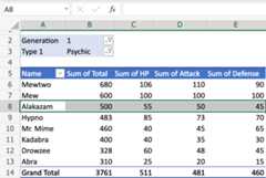
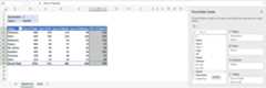
Columns are vertical tabular data.
The column includes the unique header, which is on the top.
The header defines which data you are seeing listed downwards.
In this example,D5(Sum of Attack) is the header.
D6(110), D7(100), D8(50), D9(73), and so on are the data.

Rows are horizontal tabular data.
Data in the same row are related.
In this example,A8(Alakazam) is the Pokemon name.
B8(500), C8(55), D8(50), E8(45) represents the pokemons stats.
The type of stats is read in the header in the columns.
Filters are used to select what data you see.
In this example, there are two filters enabled:Generation andType 1.
The filters are set toGeneration (1) andType (Psychic).
We will only see Generation 1 pokemon that is Type 1, Psychic.
All pokemon in the table below the filter are of this generation and type.
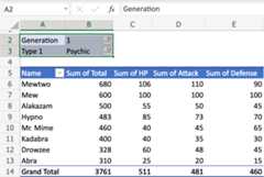
Filter view:


Values define how you present the data.
You can define how youSummarize andShow values.
In this example, values are defined for the rangeB5:E5.
The rangeB5:E5 has all the same value setting:Sum
The Sum is summarized in the rangeB14:E14.
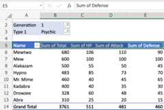
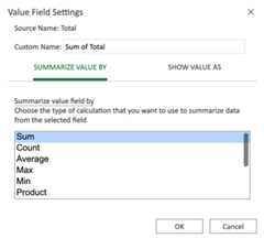
Values settings view:
You can change the name and settings of the values.
Fields and layout
The TablePivot is displayed how by your settings.
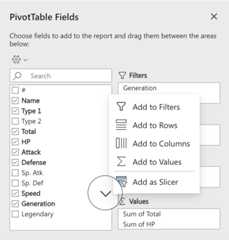
ThePivotTable Fields panel is used to change how you see the data.
The settings can be separated in two:Fields andLayout.

- Fields
- Layout
- Filters
- Rows
- Columns
- Values
The checkboxes can be selected or unselected to display or change the property of the data.
In this example, the checkbox forSpeed is selected.
Speed is now displayed in the table.
You can click the downwards arrow to change how the data is presented.
Drag and drop fields to the boxes to the right to display data in the table.
You can drag them to the four different boxes that we mentioned earlier (four main components):
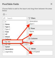
In this example, we will drag and dropSp. def toValues.

Sp. Def is now displayed in the table.
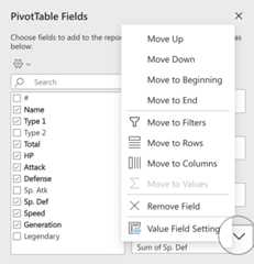
The settings of the fields that you have moved to the right side can be changed.
Click the downwards arrow to access the settings.
This is possible in the four areas (Filters, rows, columns and, values).
Chapter summary
TablePivot can be used both simple and advanced.
It can be set up in many different ways.
You can configure on many different layers cross filters, rows, columns and values.
How you set it up depends on your needs and how you want to present the data.