Download to read offline


![PrefaceThe object-relational database management system now known as PostgreSQL is derived from thePOSTGRES package written at the University of California at Berkeley. With decades of developmentbehind it, PostgreSQL is now the most advanced open-source database available anywhere.2.1. The Berkeley POSTGRES ProjectThe POSTGRES project, led by Professor Michael Stonebraker, was sponsored by the Defense Ad-vanced Research Projects Agency (DARPA), the Army Research Office (ARO), the National ScienceFoundation (NSF), and ESL, Inc. The implementation of POSTGRES began in 1986. The initial con-cepts for the system were presented in [ston86], and the definition of the initial data model appearedin [rowe87]. The design of the rule system at that time was described in [ston87a]. The rationale andarchitecture of the storage manager were detailed in [ston87b].POSTGRES has undergone several major releases since then. The first “demoware” system becameoperational in 1987 and was shown at the 1988 ACM-SIGMOD Conference. Version 1, described in[ston90a], was released to a few external users in June 1989. In response to a critique of the first rulesystem ([ston89]), the rule system was redesigned ([ston90b]), and Version 2 was released in June1990 with the new rule system. Version 3 appeared in 1991 and added support for multiple storagemanagers, an improved query executor, and a rewritten rule system. For the most part, subsequentreleases until Postgres95 (see below) focused on portability and reliability.POSTGRES has been used to implement many different research and production applications. Theseinclude: a financial data analysis system, a jet engine performance monitoring package, an aster-oid tracking database, a medical information database, and several geographic information systems.POSTGRES has also been used as an educational tool at several universities. Finally, Illustra Infor-mation Technologies (later merged into Informix2, which is now owned by IBM3) picked up the codeand commercialized it. In late 1992, POSTGRES became the primary data manager for the Sequoia2000 scientific computing project4.The size of the external user community nearly doubled during 1993. It became increasingly obviousthat maintenance of the prototype code and support was taking up large amounts of time that shouldhave been devoted to database research. In an effort to reduce this support burden, the Berkeley POST-GRES project officially ended with Version 4.2.2.2. Postgres95In 1994, Andrew Yu and Jolly Chen added an SQL language interpreter to POSTGRES. Under a newname, Postgres95 was subsequently released to the web to find its own way in the world as an open-source descendant of the original POSTGRES Berkeley code.Postgres95 code was completely ANSI C and trimmed in size by 25%. Many internal changes im-proved performance and maintainability. Postgres95 release 1.0.x ran about 30–50% faster on theWisconsin Benchmark compared to POSTGRES, Version 4.2. Apart from bug fixes, the followingwere the major enhancements:• The query language PostQUEL was replaced with SQL (implemented in the server). (Interface li-brary libpq was named after PostQUEL.) Subqueries were not supported until PostgreSQL (see be-low), but they could be imitated in Postgres95 with user-defined SQL functions. Aggregate func-tions were re-implemented. Support for the GROUP BY query clause was also added.• A new program (psql) was provided for interactive SQL queries, which used GNU Readline. Thislargely superseded the old monitor program.• A new front-end library, libpgtcl, supported Tcl-based clients. A sample shell, pgtclsh, pro-vided new Tcl commands to interface Tcl programs with the Postgres95 server.2https://www.ibm.com/analytics/informix3https://www.ibm.com/4http://meteora.ucsd.edu/s2k/s2k_home.htmlxxxiii](/image.pl?url=https%3a%2f%2fimage.slidesharecdn.com%2fpostgresql-16-a4-240621101854-e64a7806%2f85%2fpostgresql-16-3-latest-version-2024-25-pdf-33-638.jpg&f=jpg&w=240)
![Preface• The large-object interface was overhauled. The inversion large objects were the only mechanismfor storing large objects. (The inversion file system was removed.)• The instance-level rule system was removed. Rules were still available as rewrite rules.• A short tutorial introducing regular SQL features as well as those of Postgres95 was distributedwith the source code• GNU make (instead of BSD make) was used for the build. Also, Postgres95 could be compiled withan unpatched GCC (data alignment of doubles was fixed).2.3. PostgreSQLBy 1996, it became clear that the name “Postgres95” would not stand the test of time. We chose a newname, PostgreSQL, to reflect the relationship between the original POSTGRES and the more recentversions with SQL capability. At the same time, we set the version numbering to start at 6.0, puttingthe numbers back into the sequence originally begun by the Berkeley POSTGRES project.Many people continue to refer to PostgreSQL as “Postgres” (now rarely in all capital letters) becauseof tradition or because it is easier to pronounce. This usage is widely accepted as a nickname or alias.The emphasis during development of Postgres95 was on identifying and understanding existing prob-lems in the server code. With PostgreSQL, the emphasis has shifted to augmenting features and capa-bilities, although work continues in all areas.Details about what has happened in PostgreSQL since then can be found in Appendix E.3. ConventionsThe following conventions are used in the synopsis of a command: brackets ([ and ]) indicate optionalparts. Braces ({ and }) and vertical lines (|) indicate that you must choose one alternative. Dots (...)mean that the preceding element can be repeated. All other symbols, including parentheses, shouldbe taken literally.Where it enhances the clarity, SQL commands are preceded by the prompt =>, and shell commandsare preceded by the prompt $. Normally, prompts are not shown, though.An administrator is generally a person who is in charge of installing and running the server. A usercould be anyone who is using, or wants to use, any part of the PostgreSQL system. These termsshould not be interpreted too narrowly; this book does not have fixed presumptions about systemadministration procedures.4. Further InformationBesides the documentation, that is, this book, there are other resources about PostgreSQL:WikiThe PostgreSQL wiki5contains the project's FAQ6(Frequently Asked Questions) list, TODO7list, and detailed information about many more topics.Web SiteThe PostgreSQL web site8carries details on the latest release and other information to make yourwork or play with PostgreSQL more productive.5https://wiki.postgresql.org6https://wiki.postgresql.org/wiki/Frequently_Asked_Questions7https://wiki.postgresql.org/wiki/Todo8https://www.postgresql.orgxxxiv](/image.pl?url=https%3a%2f%2fimage.slidesharecdn.com%2fpostgresql-16-a4-240621101854-e64a7806%2f85%2fpostgresql-16-3-latest-version-2024-25-pdf-34-638.jpg&f=jpg&w=240)


![Chapter 2. The SQL Language2.1. IntroductionThis chapter provides an overview of how to use SQL to perform simple operations. This tutorial isonly intended to give you an introduction and is in no way a complete tutorial on SQL. Numerousbooks have been written on SQL, including [melt93] and [date97]. You should be aware that somePostgreSQL language features are extensions to the standard.In the examples that follow, we assume that you have created a database named mydb, as describedin the previous chapter, and have been able to start psql.Examples in this manual can also be found in the PostgreSQL source distribution in the directorysrc/tutorial/. (Binary distributions of PostgreSQL might not provide those files.) To use thosefiles, first change to that directory and run make:$ cd .../src/tutorial$ makeThis creates the scripts and compiles the C files containing user-defined functions and types. Then,to start the tutorial, do the following:$ psql -s mydb...mydb=> i basics.sqlThe i command reads in commands from the specified file. psql's -s option puts you in single stepmode which pauses before sending each statement to the server. The commands used in this sectionare in the file basics.sql.2.2. ConceptsPostgreSQL is a relational database management system (RDBMS). That means it is a system formanaging data stored in relations. Relation is essentially a mathematical term for table. The notionof storing data in tables is so commonplace today that it might seem inherently obvious, but thereare a number of other ways of organizing databases. Files and directories on Unix-like operating sys-tems form an example of a hierarchical database. A more modern development is the object-orienteddatabase.Each table is a named collection of rows. Each row of a given table has the same set of namedcolumns, and each column is of a specific data type. Whereas columns have a fixed order in each row,it is important to remember that SQL does not guarantee the order of the rows within the table in anyway (although they can be explicitly sorted for display).Tables are grouped into databases, and a collection of databases managed by a single PostgreSQLserver instance constitutes a database cluster.2.3. Creating a New TableYou can create a new table by specifying the table name, along with all column names and their types:7](/image.pl?url=https%3a%2f%2fimage.slidesharecdn.com%2fpostgresql-16-a4-240621101854-e64a7806%2f85%2fpostgresql-16-3-latest-version-2024-25-pdf-45-638.jpg&f=jpg&w=240)


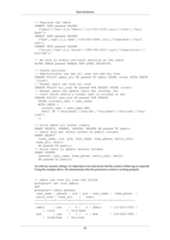
![SQL SyntaxU&'0441043B043E043D'If a different escape character than backslash is desired, it can be specified using the UESCAPE clauseafter the string, for example:U&'d!0061t!+000061' UESCAPE '!'The escape character can be any single character other than a hexadecimal digit, the plus sign, a singlequote, a double quote, or a whitespace character.To include the escape character in the string literally, write it twice.Either the 4-digit or the 6-digit escape form can be used to specify UTF-16 surrogate pairs to com-pose characters with code points larger than U+FFFF, although the availability of the 6-digit formtechnically makes this unnecessary. (Surrogate pairs are not stored directly, but are combined into asingle code point.)If the server encoding is not UTF-8, the Unicode code point identified by one of these escape sequencesis converted to the actual server encoding; an error is reported if that's not possible.Also, the Unicode escape syntax for string constants only works when the configuration parameterstandard_conforming_strings is turned on. This is because otherwise this syntax could confuse clientsthat parse the SQL statements to the point that it could lead to SQL injections and similar securityissues. If the parameter is set to off, this syntax will be rejected with an error message.4.1.2.4. Dollar-Quoted String ConstantsWhile the standard syntax for specifying string constants is usually convenient, it can be difficult tounderstand when the desired string contains many single quotes, since each of those must be doubled.To allow more readable queries in such situations, PostgreSQL provides another way, called “dollarquoting”, to write string constants. A dollar-quoted string constant consists of a dollar sign ($), anoptional “tag” of zero or more characters, another dollar sign, an arbitrary sequence of characters thatmakes up the string content, a dollar sign, the same tag that began this dollar quote, and a dollar sign.For example, here are two different ways to specify the string “Dianne's horse” using dollar quoting:$$Dianne's horse$$$SomeTag$Dianne's horse$SomeTag$Notice that inside the dollar-quoted string, single quotes can be used without needing to be escaped.Indeed, no characters inside a dollar-quoted string are ever escaped: the string content is always writtenliterally. Backslashes are not special, and neither are dollar signs, unless they are part of a sequencematching the opening tag.It is possible to nest dollar-quoted string constants by choosing different tags at each nesting level.This is most commonly used in writing function definitions. For example:$function$BEGINRETURN ($1 ~ $q$[trnv]$q$);END;$function$Here, the sequence $q$[trnv]$q$ represents a dollar-quoted literal string [trnv], which will be recognized when the function body is executed by PostgreSQL. But since thesequence does not match the outer dollar quoting delimiter $function$, it is just some more char-acters within the constant so far as the outer string is concerned.37](/image.pl?url=https%3a%2f%2fimage.slidesharecdn.com%2fpostgresql-16-a4-240621101854-e64a7806%2f85%2fpostgresql-16-3-latest-version-2024-25-pdf-75-638.jpg&f=jpg&w=240)
![SQL SyntaxThe tag, if any, of a dollar-quoted string follows the same rules as an unquoted identifier, except that itcannot contain a dollar sign. Tags are case sensitive, so $tag$String content$tag$ is correct,but $TAG$String content$tag$ is not.A dollar-quoted string that follows a keyword or identifier must be separated from it by whitespace;otherwise the dollar quoting delimiter would be taken as part of the preceding identifier.Dollar quoting is not part of the SQL standard, but it is often a more convenient way to write com-plicated string literals than the standard-compliant single quote syntax. It is particularly useful whenrepresenting string constants inside other constants, as is often needed in procedural function defini-tions. With single-quote syntax, each backslash in the above example would have to be written as fourbackslashes, which would be reduced to two backslashes in parsing the original string constant, andthen to one when the inner string constant is re-parsed during function execution.4.1.2.5. Bit-String ConstantsBit-string constants look like regular string constants with a B (upper or lower case) immediatelybefore the opening quote (no intervening whitespace), e.g., B'1001'. The only characters allowedwithin bit-string constants are 0 and 1.Alternatively, bit-string constants can be specified in hexadecimal notation, using a leading X (upperor lower case), e.g., X'1FF'. This notation is equivalent to a bit-string constant with four binary digitsfor each hexadecimal digit.Both forms of bit-string constant can be continued across lines in the same way as regular stringconstants. Dollar quoting cannot be used in a bit-string constant.4.1.2.6. Numeric ConstantsNumeric constants are accepted in these general forms:digitsdigits.[digits][e[+-]digits][digits].digits[e[+-]digits]digitse[+-]digitswhere digits is one or more decimal digits (0 through 9). At least one digit must be before orafter the decimal point, if one is used. At least one digit must follow the exponent marker (e), ifone is present. There cannot be any spaces or other characters embedded in the constant, except forunderscores, which can be used for visual grouping as described below. Note that any leading plus orminus sign is not actually considered part of the constant; it is an operator applied to the constant.These are some examples of valid numeric constants:423.54..0015e21.925e-3Additionally, non-decimal integer constants are accepted in these forms:0xhexdigits0ooctdigits0bbindigits38](/image.pl?url=https%3a%2f%2fimage.slidesharecdn.com%2fpostgresql-16-a4-240621101854-e64a7806%2f85%2fpostgresql-16-3-latest-version-2024-25-pdf-76-638.jpg&f=jpg&w=240)

![SQL SyntaxIt is also possible to specify a type coercion using a function-like syntax:typename ( 'string' )but not all type names can be used in this way; see Section 4.2.9 for details.The ::, CAST(), and function-call syntaxes can also be used to specify run-time type conver-sions of arbitrary expressions, as discussed in Section 4.2.9. To avoid syntactic ambiguity, the type'string' syntax can only be used to specify the type of a simple literal constant. Another restrictionon the type 'string' syntax is that it does not work for array types; use :: or CAST() to specifythe type of an array constant.The CAST() syntax conforms to SQL. The type 'string' syntax is a generalization of thestandard: SQL specifies this syntax only for a few data types, but PostgreSQL allows it for all types.The syntax with :: is historical PostgreSQL usage, as is the function-call syntax.4.1.3. OperatorsAn operator name is a sequence of up to NAMEDATALEN-1 (63 by default) characters from the fol-lowing list:+ - * / < > = ~ ! @ # % ^ & | ` ?There are a few restrictions on operator names, however:• -- and /* cannot appear anywhere in an operator name, since they will be taken as the start ofa comment.• A multiple-character operator name cannot end in + or -, unless the name also contains at leastone of these characters:~ ! @ # % ^ & | ` ?For example, @- is an allowed operator name, but *- is not. This restriction allows PostgreSQL toparse SQL-compliant queries without requiring spaces between tokens.When working with non-SQL-standard operator names, you will usually need to separate adjacentoperators with spaces to avoid ambiguity. For example, if you have defined a prefix operator named@, you cannot write X*@Y; you must write X* @Y to ensure that PostgreSQL reads it as two operatornames not one.4.1.4. Special CharactersSome characters that are not alphanumeric have a special meaning that is different from being an oper-ator. Details on the usage can be found at the location where the respective syntax element is described.This section only exists to advise the existence and summarize the purposes of these characters.• A dollar sign ($) followed by digits is used to represent a positional parameter in the body of afunction definition or a prepared statement. In other contexts the dollar sign can be part of an iden-tifier or a dollar-quoted string constant.• Parentheses (()) have their usual meaning to group expressions and enforce precedence. In somecases parentheses are required as part of the fixed syntax of a particular SQL command.• Brackets ([]) are used to select the elements of an array. See Section 8.15 for more informationon arrays.• Commas (,) are used in some syntactical constructs to separate the elements of a list.40](/image.pl?url=https%3a%2f%2fimage.slidesharecdn.com%2fpostgresql-16-a4-240621101854-e64a7806%2f85%2fpostgresql-16-3-latest-version-2024-25-pdf-78-638.jpg&f=jpg&w=240)
![SQL Syntax• The semicolon (;) terminates an SQL command. It cannot appear anywhere within a command,except within a string constant or quoted identifier.• The colon (:) is used to select “slices” from arrays. (See Section 8.15.) In certain SQL dialects(such as Embedded SQL), the colon is used to prefix variable names.• The asterisk (*) is used in some contexts to denote all the fields of a table row or composite value.It also has a special meaning when used as the argument of an aggregate function, namely that theaggregate does not require any explicit parameter.• The period (.) is used in numeric constants, and to separate schema, table, and column names.4.1.5. CommentsA comment is a sequence of characters beginning with double dashes and extending to the end ofthe line, e.g.:-- This is a standard SQL commentAlternatively, C-style block comments can be used:/* multiline comment* with nesting: /* nested block comment */*/where the comment begins with /* and extends to the matching occurrence of */. These block com-ments nest, as specified in the SQL standard but unlike C, so that one can comment out larger blocksof code that might contain existing block comments.A comment is removed from the input stream before further syntax analysis and is effectively replacedby whitespace.4.1.6. Operator PrecedenceTable 4.2 shows the precedence and associativity of the operators in PostgreSQL. Most operators havethe same precedence and are left-associative. The precedence and associativity of the operators is hard-wired into the parser. Add parentheses if you want an expression with multiple operators to be parsedin some other way than what the precedence rules imply.Table 4.2. Operator Precedence (highest to lowest)Operator/Element Associativity Description. left table/column name separator:: left PostgreSQL-style typecast[ ] left array element selection+ - right unary plus, unary minusCOLLATE left collation selectionAT left AT TIME ZONE^ left exponentiation* / % left multiplication, division, modulo+ - left addition, subtraction(any other operator) left all other native and user-defined oper-ators41](/image.pl?url=https%3a%2f%2fimage.slidesharecdn.com%2fpostgresql-16-a4-240621101854-e64a7806%2f85%2fpostgresql-16-3-latest-version-2024-25-pdf-79-638.jpg&f=jpg&w=240)


![SQL Syntaxexpression[subscript]or multiple adjacent elements (an “array slice”) can be extracted by writingexpression[lower_subscript:upper_subscript](Here, the brackets [ ] are meant to appear literally.) Each subscript is itself an expression, whichwill be rounded to the nearest integer value.In general the array expression must be parenthesized, but the parentheses can be omitted whenthe expression to be subscripted is just a column reference or positional parameter. Also, multiplesubscripts can be concatenated when the original array is multidimensional. For example:mytable.arraycolumn[4]mytable.two_d_column[17][34]$1[10:42](arrayfunction(a,b))[42]The parentheses in the last example are required. See Section 8.15 for more about arrays.4.2.4. Field SelectionIf an expression yields a value of a composite type (row type), then a specific field of the row canbe extracted by writingexpression.fieldnameIn general the row expression must be parenthesized, but the parentheses can be omitted when theexpression to be selected from is just a table reference or positional parameter. For example:mytable.mycolumn$1.somecolumn(rowfunction(a,b)).col3(Thus, a qualified column reference is actually just a special case of the field selection syntax.) Animportant special case is extracting a field from a table column that is of a composite type:(compositecol).somefield(mytable.compositecol).somefieldThe parentheses are required here to show that compositecol is a column name not a table name,or that mytable is a table name not a schema name in the second case.You can ask for all fields of a composite value by writing .*:(compositecol).*This notation behaves differently depending on context; see Section 8.16.5 for details.4.2.5. Operator InvocationsThere are two possible syntaxes for an operator invocation:expression operator expression (binary infix operator)44](/image.pl?url=https%3a%2f%2fimage.slidesharecdn.com%2fpostgresql-16-a4-240621101854-e64a7806%2f85%2fpostgresql-16-3-latest-version-2024-25-pdf-82-638.jpg&f=jpg&w=240)
![SQL Syntaxoperator expression (unary prefix operator)where the operator token follows the syntax rules of Section 4.1.3, or is one of the key words AND,OR, and NOT, or is a qualified operator name in the form:OPERATOR(schema.operatorname)Which particular operators exist and whether they are unary or binary depends on what operators havebeen defined by the system or the user. Chapter 9 describes the built-in operators.4.2.6. Function CallsThe syntax for a function call is the name of a function (possibly qualified with a schema name),followed by its argument list enclosed in parentheses:function_name ([expression [, expression ... ]] )For example, the following computes the square root of 2:sqrt(2)The list of built-in functions is in Chapter 9. Other functions can be added by the user.When issuing queries in a database where some users mistrust other users, observe security precautionsfrom Section 10.3 when writing function calls.The arguments can optionally have names attached. See Section 4.3 for details.NoteA function that takes a single argument of composite type can optionally be called using field-selection syntax, and conversely field selection can be written in functional style. That is, thenotations col(table) and table.col are interchangeable. This behavior is not SQL-standard but is provided in PostgreSQL because it allows use of functions to emulate “com-puted fields”. For more information see Section 8.16.5.4.2.7. Aggregate ExpressionsAn aggregate expression represents the application of an aggregate function across the rows selectedby a query. An aggregate function reduces multiple inputs to a single output value, such as the sum oraverage of the inputs. The syntax of an aggregate expression is one of the following:aggregate_name (expression [ , ... ] [ order_by_clause ] ) [ FILTER( WHERE filter_clause ) ]aggregate_name (ALL expression [ , ... ] [ order_by_clause ] )[ FILTER ( WHERE filter_clause ) ]aggregate_name (DISTINCT expression [ , ... ] [ order_by_clause ] )[ FILTER ( WHERE filter_clause ) ]aggregate_name ( * ) [ FILTER ( WHERE filter_clause ) ]aggregate_name ( [ expression [ , ... ] ] ) WITHIN GROUP( order_by_clause ) [ FILTER ( WHERE filter_clause ) ]where aggregate_name is a previously defined aggregate (possibly qualified with a schema name)and expression is any value expression that does not itself contain an aggregate expression or45](/image.pl?url=https%3a%2f%2fimage.slidesharecdn.com%2fpostgresql-16-a4-240621101854-e64a7806%2f85%2fpostgresql-16-3-latest-version-2024-25-pdf-83-638.jpg&f=jpg&w=240)


![SQL Syntaxselected rows into a single output row — each row remains separate in the query output. However thewindow function has access to all the rows that would be part of the current row's group accordingto the grouping specification (PARTITION BY list) of the window function call. The syntax of awindow function call is one of the following:function_name ([expression [, expression ... ]]) [ FILTER( WHERE filter_clause ) ] OVER window_namefunction_name ([expression [, expression ... ]]) [ FILTER( WHERE filter_clause ) ] OVER ( window_definition )function_name ( * ) [ FILTER ( WHERE filter_clause ) ]OVER window_namefunction_name ( * ) [ FILTER ( WHERE filter_clause ) ] OVER( window_definition )where window_definition has the syntax[ existing_window_name ][ PARTITION BY expression [, ...] ][ ORDER BY expression [ ASC | DESC | USING operator ] [ NULLS{ FIRST | LAST } ] [, ...] ][ frame_clause ]The optional frame_clause can be one of{ RANGE | ROWS | GROUPS } frame_start [ frame_exclusion ]{ RANGE | ROWS | GROUPS } BETWEEN frame_start AND frame_end[ frame_exclusion ]where frame_start and frame_end can be one ofUNBOUNDED PRECEDINGoffset PRECEDINGCURRENT ROWoffset FOLLOWINGUNBOUNDED FOLLOWINGand frame_exclusion can be one ofEXCLUDE CURRENT ROWEXCLUDE GROUPEXCLUDE TIESEXCLUDE NO OTHERSHere, expression represents any value expression that does not itself contain window functioncalls.window_name is a reference to a named window specification defined in the query's WINDOW clause.Alternatively, a full window_definition can be given within parentheses, using the same syntaxas for defining a named window in the WINDOW clause; see the SELECT reference page for details. It'sworth pointing out that OVER wname is not exactly equivalent to OVER (wname ...); the latterimplies copying and modifying the window definition, and will be rejected if the referenced windowspecification includes a frame clause.The PARTITION BY clause groups the rows of the query into partitions, which are processed sepa-rately by the window function. PARTITION BY works similarly to a query-level GROUP BY clause,48](/image.pl?url=https%3a%2f%2fimage.slidesharecdn.com%2fpostgresql-16-a4-240621101854-e64a7806%2f85%2fpostgresql-16-3-latest-version-2024-25-pdf-86-638.jpg&f=jpg&w=240)


![SQL Syntax4.2.11. Scalar SubqueriesA scalar subquery is an ordinary SELECT query in parentheses that returns exactly one row with onecolumn. (See Chapter 7 for information about writing queries.) The SELECT query is executed andthe single returned value is used in the surrounding value expression. It is an error to use a query thatreturns more than one row or more than one column as a scalar subquery. (But if, during a particularexecution, the subquery returns no rows, there is no error; the scalar result is taken to be null.) Thesubquery can refer to variables from the surrounding query, which will act as constants during anyone evaluation of the subquery. See also Section 9.23 for other expressions involving subqueries.For example, the following finds the largest city population in each state:SELECT name, (SELECT max(pop) FROM cities WHERE cities.state =states.name)FROM states;4.2.12. Array ConstructorsAn array constructor is an expression that builds an array value using values for its member elements. Asimple array constructor consists of the key word ARRAY, a left square bracket [, a list of expressions(separated by commas) for the array element values, and finally a right square bracket ]. For example:SELECT ARRAY[1,2,3+4];array---------{1,2,7}(1 row)By default, the array element type is the common type of the member expressions, determined usingthe same rules as for UNION or CASE constructs (see Section 10.5). You can override this by explicitlycasting the array constructor to the desired type, for example:SELECT ARRAY[1,2,22.7]::integer[];array----------{1,2,23}(1 row)This has the same effect as casting each expression to the array element type individually. For moreon casting, see Section 4.2.9.Multidimensional array values can be built by nesting array constructors. In the inner constructors, thekey word ARRAY can be omitted. For example, these produce the same result:SELECT ARRAY[ARRAY[1,2], ARRAY[3,4]];array---------------{{1,2},{3,4}}(1 row)SELECT ARRAY[[1,2],[3,4]];array---------------{{1,2},{3,4}}(1 row)52](/image.pl?url=https%3a%2f%2fimage.slidesharecdn.com%2fpostgresql-16-a4-240621101854-e64a7806%2f85%2fpostgresql-16-3-latest-version-2024-25-pdf-90-638.jpg&f=jpg&w=240)
![SQL SyntaxSince multidimensional arrays must be rectangular, inner constructors at the same level must producesub-arrays of identical dimensions. Any cast applied to the outer ARRAY constructor propagates au-tomatically to all the inner constructors.Multidimensional array constructor elements can be anything yielding an array of the proper kind, notonly a sub-ARRAY construct. For example:CREATE TABLE arr(f1 int[], f2 int[]);INSERT INTO arr VALUES (ARRAY[[1,2],[3,4]], ARRAY[[5,6],[7,8]]);SELECT ARRAY[f1, f2, '{{9,10},{11,12}}'::int[]] FROM arr;array------------------------------------------------{{{1,2},{3,4}},{{5,6},{7,8}},{{9,10},{11,12}}}(1 row)You can construct an empty array, but since it's impossible to have an array with no type, you mustexplicitly cast your empty array to the desired type. For example:SELECT ARRAY[]::integer[];array-------{}(1 row)It is also possible to construct an array from the results of a subquery. In this form, the array construc-tor is written with the key word ARRAY followed by a parenthesized (not bracketed) subquery. Forexample:SELECT ARRAY(SELECT oid FROM pg_proc WHERE proname LIKE 'bytea%');array------------------------------------------------------------------{2011,1954,1948,1952,1951,1244,1950,2005,1949,1953,2006,31,2412}(1 row)SELECT ARRAY(SELECT ARRAY[i, i*2] FROM generate_series(1,5) ASa(i));array----------------------------------{{1,2},{2,4},{3,6},{4,8},{5,10}}(1 row)The subquery must return a single column. If the subquery's output column is of a non-array type,the resulting one-dimensional array will have an element for each row in the subquery result, with anelement type matching that of the subquery's output column. If the subquery's output column is of anarray type, the result will be an array of the same type but one higher dimension; in this case all thesubquery rows must yield arrays of identical dimensionality, else the result would not be rectangular.The subscripts of an array value built with ARRAY always begin with one. For more information aboutarrays, see Section 8.15.4.2.13. Row ConstructorsA row constructor is an expression that builds a row value (also called a composite value) using valuesfor its member fields. A row constructor consists of the key word ROW, a left parenthesis, zero or53](/image.pl?url=https%3a%2f%2fimage.slidesharecdn.com%2fpostgresql-16-a4-240621101854-e64a7806%2f85%2fpostgresql-16-3-latest-version-2024-25-pdf-91-638.jpg&f=jpg&w=240)


![Data DefinitionObject Type All Privileges Default PUBLICPrivilegespsql CommandPARAMETER sA none dconfig+SCHEMA UC none dn+SEQUENCE rwU none dpTABLE (and table-like objects) arwdDxt none dpTable column arwx none dpTABLESPACE C none db+TYPE U U dT+The privileges that have been granted for a particular object are displayed as a list of aclitementries, each having the format:grantee=privilege-abbreviation[*].../grantorEach aclitem lists all the permissions of one grantee that have been granted by a particular grantor.Specific privileges are represented by one-letter abbreviations from Table 5.1, with * appended if theprivilege was granted with grant option. For example, calvin=r*w/hobbes specifies that the rolecalvin has the privilege SELECT (r) with grant option (*) as well as the non-grantable privilegeUPDATE (w), both granted by the role hobbes. If calvin also has some privileges on the sameobject granted by a different grantor, those would appear as a separate aclitem entry. An emptygrantee field in an aclitem stands for PUBLIC.As an example, suppose that user miriam creates table mytable and does:GRANT SELECT ON mytable TO PUBLIC;GRANT SELECT, UPDATE, INSERT ON mytable TO admin;GRANT SELECT (col1), UPDATE (col1) ON mytable TO miriam_rw;Then psql's dp command would show:=> dp mytableAccess privilegesSchema | Name | Type | Access privileges | Columnprivileges | Policies--------+---------+-------+-----------------------+-----------------------+----------public | mytable | table | miriam=arwdDxt/miriam+| col1:+|| | | =r/miriam +| miriam_rw=rw/miriam || | | admin=arw/miriam ||(1 row)If the “Access privileges” column is empty for a given object, it means the object has default privileges(that is, its privileges entry in the relevant system catalog is null). Default privileges always include allprivileges for the owner, and can include some privileges for PUBLIC depending on the object type,as explained above. The first GRANT or REVOKE on an object will instantiate the default privileges(producing, for example, miriam=arwdDxt/miriam) and then modify them per the specified re-quest. Similarly, entries are shown in “Column privileges” only for columns with nondefault privi-leges. (Note: for this purpose, “default privileges” always means the built-in default privileges for theobject's type. An object whose privileges have been affected by an ALTER DEFAULT PRIVILEGEScommand will always be shown with an explicit privilege entry that includes the effects of the ALTER.)79](/image.pl?url=https%3a%2f%2fimage.slidesharecdn.com%2fpostgresql-16-a4-240621101854-e64a7806%2f85%2fpostgresql-16-3-latest-version-2024-25-pdf-117-638.jpg&f=jpg&w=240)


![Chapter 7. QueriesThe previous chapters explained how to create tables, how to fill them with data, and how to manipulatethat data. Now we finally discuss how to retrieve the data from the database.7.1. OverviewThe process of retrieving or the command to retrieve data from a database is called a query. In SQLthe SELECT command is used to specify queries. The general syntax of the SELECT command is[WITH with_queries] SELECT select_list FROM table_expression[sort_specification]The following sections describe the details of the select list, the table expression, and the sort specifi-cation. WITH queries are treated last since they are an advanced feature.A simple kind of query has the form:SELECT * FROM table1;Assuming that there is a table called table1, this command would retrieve all rows and all user-defined columns from table1. (The method of retrieval depends on the client application. For ex-ample, the psql program will display an ASCII-art table on the screen, while client libraries will offerfunctions to extract individual values from the query result.) The select list specification * means allcolumns that the table expression happens to provide. A select list can also select a subset of the avail-able columns or make calculations using the columns. For example, if table1 has columns nameda, b, and c (and perhaps others) you can make the following query:SELECT a, b + c FROM table1;(assuming that b and c are of a numerical data type). See Section 7.3 for more details.FROM table1 is a simple kind of table expression: it reads just one table. In general, table expres-sions can be complex constructs of base tables, joins, and subqueries. But you can also omit the tableexpression entirely and use the SELECT command as a calculator:SELECT 3 * 4;This is more useful if the expressions in the select list return varying results. For example, you couldcall a function this way:SELECT random();7.2. Table ExpressionsA table expression computes a table. The table expression contains a FROM clause that is optionallyfollowed by WHERE, GROUP BY, and HAVING clauses. Trivial table expressions simply refer to atable on disk, a so-called base table, but more complex expressions can be used to modify or combinebase tables in various ways.The optional WHERE, GROUP BY, and HAVING clauses in the table expression specify a pipeline ofsuccessive transformations performed on the table derived in the FROM clause. All these transforma-115](/image.pl?url=https%3a%2f%2fimage.slidesharecdn.com%2fpostgresql-16-a4-240621101854-e64a7806%2f85%2fpostgresql-16-3-latest-version-2024-25-pdf-153-638.jpg&f=jpg&w=240)
![Queriestions produce a virtual table that provides the rows that are passed to the select list to compute theoutput rows of the query.7.2.1. The FROM ClauseThe FROM clause derives a table from one or more other tables given in a comma-separated tablereference list.FROM table_reference [, table_reference [, ...]]A table reference can be a table name (possibly schema-qualified), or a derived table such as a sub-query, a JOIN construct, or complex combinations of these. If more than one table reference is listedin the FROM clause, the tables are cross-joined (that is, the Cartesian product of their rows is formed;see below). The result of the FROM list is an intermediate virtual table that can then be subject to trans-formations by the WHERE, GROUP BY, and HAVING clauses and is finally the result of the overalltable expression.When a table reference names a table that is the parent of a table inheritance hierarchy, the tablereference produces rows of not only that table but all of its descendant tables, unless the key wordONLY precedes the table name. However, the reference produces only the columns that appear in thenamed table — any columns added in subtables are ignored.Instead of writing ONLY before the table name, you can write * after the table name to explicitlyspecify that descendant tables are included. There is no real reason to use this syntax any more, be-cause searching descendant tables is now always the default behavior. However, it is supported forcompatibility with older releases.7.2.1.1. Joined TablesA joined table is a table derived from two other (real or derived) tables according to the rules of theparticular join type. Inner, outer, and cross-joins are available. The general syntax of a joined table isT1 join_type T2 [ join_condition ]Joins of all types can be chained together, or nested: either or both T1 and T2 can be joined tables.Parentheses can be used around JOIN clauses to control the join order. In the absence of parentheses,JOIN clauses nest left-to-right.Join TypesCross joinT1 CROSS JOIN T2For every possible combination of rows from T1 and T2 (i.e., a Cartesian product), the joinedtable will contain a row consisting of all columns in T1 followed by all columns in T2. If thetables have N and M rows respectively, the joined table will have N * M rows.FROM T1 CROSS JOIN T2 is equivalent to FROM T1 INNER JOIN T2 ON TRUE (seebelow). It is also equivalent to FROM T1, T2.NoteThis latter equivalence does not hold exactly when more than two tables appear, becauseJOIN binds more tightly than comma. For example FROM T1 CROSS JOIN T2INNER JOIN T3 ON condition is not the same as FROM T1, T2 INNER JOIN116](/image.pl?url=https%3a%2f%2fimage.slidesharecdn.com%2fpostgresql-16-a4-240621101854-e64a7806%2f85%2fpostgresql-16-3-latest-version-2024-25-pdf-154-638.jpg&f=jpg&w=240)
![QueriesT3 ON condition because the condition can reference T1 in the first case butnot the second.Qualified joinsT1 { [INNER] | { LEFT | RIGHT | FULL } [OUTER] } JOIN T2ON boolean_expressionT1 { [INNER] | { LEFT | RIGHT | FULL } [OUTER] } JOIN T2 USING( join column list )T1 NATURAL { [INNER] | { LEFT | RIGHT | FULL } [OUTER] } JOIN T2The words INNER and OUTER are optional in all forms. INNER is the default; LEFT, RIGHT,and FULL imply an outer join.The join condition is specified in the ON or USING clause, or implicitly by the word NATURAL.The join condition determines which rows from the two source tables are considered to “match”,as explained in detail below.The possible types of qualified join are:INNER JOINFor each row R1 of T1, the joined table has a row for each row in T2 that satisfies the joincondition with R1.LEFT OUTER JOINFirst, an inner join is performed. Then, for each row in T1 that does not satisfy the joincondition with any row in T2, a joined row is added with null values in columns of T2. Thus,the joined table always has at least one row for each row in T1.RIGHT OUTER JOINFirst, an inner join is performed. Then, for each row in T2 that does not satisfy the joincondition with any row in T1, a joined row is added with null values in columns of T1. Thisis the converse of a left join: the result table will always have a row for each row in T2.FULL OUTER JOINFirst, an inner join is performed. Then, for each row in T1 that does not satisfy the joincondition with any row in T2, a joined row is added with null values in columns of T2. Also,for each row of T2 that does not satisfy the join condition with any row in T1, a joined rowwith null values in the columns of T1 is added.The ON clause is the most general kind of join condition: it takes a Boolean value expression ofthe same kind as is used in a WHERE clause. A pair of rows from T1 and T2 match if the ONexpression evaluates to true.The USING clause is a shorthand that allows you to take advantage of the specific situation whereboth sides of the join use the same name for the joining column(s). It takes a comma-separatedlist of the shared column names and forms a join condition that includes an equality comparisonfor each one. For example, joining T1 and T2 with USING (a, b) produces the join conditionON T1.a = T2.a AND T1.b = T2.b.Furthermore, the output of JOIN USING suppresses redundant columns: there is no need to printboth of the matched columns, since they must have equal values. While JOIN ON produces allcolumns from T1 followed by all columns from T2, JOIN USING produces one output columnfor each of the listed column pairs (in the listed order), followed by any remaining columns fromT1, followed by any remaining columns from T2.117](/image.pl?url=https%3a%2f%2fimage.slidesharecdn.com%2fpostgresql-16-a4-240621101854-e64a7806%2f85%2fpostgresql-16-3-latest-version-2024-25-pdf-155-638.jpg&f=jpg&w=240)


![Queries=> SELECT * FROM t1 LEFT JOIN t2 ON t1.num = t2.num WHERE t2.value= 'xxx';num | name | num | value-----+------+-----+-------1 | a | 1 | xxx(1 row)This is because a restriction placed in the ON clause is processed before the join, while a restrictionplaced in the WHERE clause is processed after the join. That does not matter with inner joins, but itmatters a lot with outer joins.7.2.1.2. Table and Column AliasesA temporary name can be given to tables and complex table references to be used for references tothe derived table in the rest of the query. This is called a table alias.To create a table alias, writeFROM table_reference AS aliasorFROM table_reference aliasThe AS key word is optional noise. alias can be any identifier.A typical application of table aliases is to assign short identifiers to long table names to keep the joinclauses readable. For example:SELECT * FROM some_very_long_table_name s JOINanother_fairly_long_name a ON s.id = a.num;The alias becomes the new name of the table reference so far as the current query is concerned — itis not allowed to refer to the table by the original name elsewhere in the query. Thus, this is not valid:SELECT * FROM my_table AS m WHERE my_table.a > 5; -- wrongTable aliases are mainly for notational convenience, but it is necessary to use them when joining atable to itself, e.g.:SELECT * FROM people AS mother JOIN people AS child ON mother.id =child.mother_id;Parentheses are used to resolve ambiguities. In the following example, the first statement assigns thealias b to the second instance of my_table, but the second statement assigns the alias to the resultof the join:SELECT * FROM my_table AS a CROSS JOIN my_table AS b ...SELECT * FROM (my_table AS a CROSS JOIN my_table) AS b ...Another form of table aliasing gives temporary names to the columns of the table, as well as the tableitself:FROM table_reference [AS] alias ( column1 [, column2 [, ...]] )120](/image.pl?url=https%3a%2f%2fimage.slidesharecdn.com%2fpostgresql-16-a4-240621101854-e64a7806%2f85%2fpostgresql-16-3-latest-version-2024-25-pdf-158-638.jpg&f=jpg&w=240)
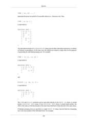
![QueriesIf fewer column aliases are specified than the actual table has columns, the remaining columns are notrenamed. This syntax is especially useful for self-joins or subqueries.When an alias is applied to the output of a JOIN clause, the alias hides the original name(s) withinthe JOIN. For example:SELECT a.* FROM my_table AS a JOIN your_table AS b ON ...is valid SQL, but:SELECT a.* FROM (my_table AS a JOIN your_table AS b ON ...) AS cis not valid; the table alias a is not visible outside the alias c.7.2.1.3. SubqueriesSubqueries specifying a derived table must be enclosed in parentheses. They may be assigned a tablealias name, and optionally column alias names (as in Section 7.2.1.2). For example:FROM (SELECT * FROM table1) AS alias_nameThis example is equivalent to FROM table1 AS alias_name. More interesting cases, whichcannot be reduced to a plain join, arise when the subquery involves grouping or aggregation.A subquery can also be a VALUES list:FROM (VALUES ('anne', 'smith'), ('bob', 'jones'), ('joe', 'blow'))AS names(first, last)Again, a table alias is optional. Assigning alias names to the columns of the VALUES list is optional,but is good practice. For more information see Section 7.7.According to the SQL standard, a table alias name must be supplied for a subquery. PostgreSQL allowsAS and the alias to be omitted, but writing one is good practice in SQL code that might be ported toanother system.7.2.1.4. Table FunctionsTable functions are functions that produce a set of rows, made up of either base data types (scalartypes) or composite data types (table rows). They are used like a table, view, or subquery in the FROMclause of a query. Columns returned by table functions can be included in SELECT, JOIN, or WHEREclauses in the same manner as columns of a table, view, or subquery.Table functions may also be combined using the ROWS FROM syntax, with the results returned inparallel columns; the number of result rows in this case is that of the largest function result, withsmaller results padded with null values to match.function_call [WITH ORDINALITY] [[AS] table_alias [(column_alias[, ... ])]]ROWS FROM( function_call [, ... ] ) [WITH ORDINALITY][[AS] table_alias [(column_alias [, ... ])]]If the WITH ORDINALITY clause is specified, an additional column of type bigint will be addedto the function result columns. This column numbers the rows of the function result set, starting from1. (This is a generalization of the SQL-standard syntax for UNNEST ... WITH ORDINALITY.)121](/image.pl?url=https%3a%2f%2fimage.slidesharecdn.com%2fpostgresql-16-a4-240621101854-e64a7806%2f85%2fpostgresql-16-3-latest-version-2024-25-pdf-159-638.jpg&f=jpg&w=240)
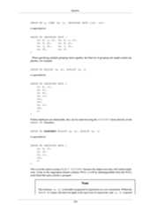
![QueriesBy default, the ordinal column is called ordinality, but a different column name can be assignedto it using an AS clause.The special table function UNNEST may be called with any number of array parameters, and it returnsa corresponding number of columns, as if UNNEST (Section 9.19) had been called on each parameterseparately and combined using the ROWS FROM construct.UNNEST( array_expression [, ... ] ) [WITH ORDINALITY][[AS] table_alias [(column_alias [, ... ])]]If no table_alias is specified, the function name is used as the table name; in the case of a ROWSFROM() construct, the first function's name is used.If column aliases are not supplied, then for a function returning a base data type, the column name isalso the same as the function name. For a function returning a composite type, the result columns getthe names of the individual attributes of the type.Some examples:CREATE TABLE foo (fooid int, foosubid int, fooname text);CREATE FUNCTION getfoo(int) RETURNS SETOF foo AS $$SELECT * FROM foo WHERE fooid = $1;$$ LANGUAGE SQL;SELECT * FROM getfoo(1) AS t1;SELECT * FROM fooWHERE foosubid IN (SELECT foosubidFROM getfoo(foo.fooid) zWHERE z.fooid = foo.fooid);CREATE VIEW vw_getfoo AS SELECT * FROM getfoo(1);SELECT * FROM vw_getfoo;In some cases it is useful to define table functions that can return different column sets depending onhow they are invoked. To support this, the table function can be declared as returning the pseudo-typerecord with no OUT parameters. When such a function is used in a query, the expected row structuremust be specified in the query itself, so that the system can know how to parse and plan the query.This syntax looks like:function_call [AS] alias (column_definition [, ... ])function_call AS [alias] (column_definition [, ... ])ROWS FROM( ... function_call AS (column_definition [, ... ])[, ... ] )When not using the ROWS FROM() syntax, the column_definition list replaces the columnalias list that could otherwise be attached to the FROM item; the names in the column definitions serveas column aliases. When using the ROWS FROM() syntax, a column_definition list can beattached to each member function separately; or if there is only one member function and no WITHORDINALITY clause, a column_definition list can be written in place of a column alias listfollowing ROWS FROM().Consider this example:122](/image.pl?url=https%3a%2f%2fimage.slidesharecdn.com%2fpostgresql-16-a4-240621101854-e64a7806%2f85%2fpostgresql-16-3-latest-version-2024-25-pdf-160-638.jpg&f=jpg&w=240)
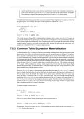
![QueriesSELECT *FROM dblink('dbname=mydb', 'SELECT proname, prosrc FROMpg_proc')AS t1(proname name, prosrc text)WHERE proname LIKE 'bytea%';The dblink function (part of the dblink module) executes a remote query. It is declared to returnrecord since it might be used for any kind of query. The actual column set must be specified in thecalling query so that the parser knows, for example, what * should expand to.This example uses ROWS FROM:SELECT *FROM ROWS FROM(json_to_recordset('[{"a":40,"b":"foo"},{"a":"100","b":"bar"}]')AS (a INTEGER, b TEXT),generate_series(1, 3)) AS x (p, q, s)ORDER BY p;p | q | s-----+-----+---40 | foo | 1100 | bar | 2| | 3It joins two functions into a single FROM target. json_to_recordset() is instructed to returntwo columns, the first integer and the second text. The result of generate_series() is useddirectly. The ORDER BY clause sorts the column values as integers.7.2.1.5. LATERAL SubqueriesSubqueries appearing in FROM can be preceded by the key word LATERAL. This allows them to ref-erence columns provided by preceding FROM items. (Without LATERAL, each subquery is evaluatedindependently and so cannot cross-reference any other FROM item.)Table functions appearing in FROM can also be preceded by the key word LATERAL, but for functionsthe key word is optional; the function's arguments can contain references to columns provided bypreceding FROM items in any case.A LATERAL item can appear at the top level in the FROM list, or within a JOIN tree. In the latter caseit can also refer to any items that are on the left-hand side of a JOIN that it is on the right-hand side of.When a FROM item contains LATERAL cross-references, evaluation proceeds as follows: for eachrow of the FROM item providing the cross-referenced column(s), or set of rows of multiple FROMitems providing the columns, the LATERAL item is evaluated using that row or row set's values ofthe columns. The resulting row(s) are joined as usual with the rows they were computed from. This isrepeated for each row or set of rows from the column source table(s).A trivial example of LATERAL isSELECT * FROM foo, LATERAL (SELECT * FROM bar WHERE bar.id =foo.bar_id) ss;This is not especially useful since it has exactly the same result as the more conventional123](/image.pl?url=https%3a%2f%2fimage.slidesharecdn.com%2fpostgresql-16-a4-240621101854-e64a7806%2f85%2fpostgresql-16-3-latest-version-2024-25-pdf-161-638.jpg&f=jpg&w=240)

![QueriesFROM a, b WHERE a.id = b.id AND b.val > 5and:FROM a INNER JOIN b ON (a.id = b.id) WHERE b.val > 5or perhaps even:FROM a NATURAL JOIN b WHERE b.val > 5Which one of these you use is mainly a matter of style. The JOIN syntax in the FROM clauseis probably not as portable to other SQL database management systems, even though it is inthe SQL standard. For outer joins there is no choice: they must be done in the FROM clause.The ON or USING clause of an outer join is not equivalent to a WHERE condition, becauseit results in the addition of rows (for unmatched input rows) as well as the removal of rowsin the final result.Here are some examples of WHERE clauses:SELECT ... FROM fdt WHERE c1 > 5SELECT ... FROM fdt WHERE c1 IN (1, 2, 3)SELECT ... FROM fdt WHERE c1 IN (SELECT c1 FROM t2)SELECT ... FROM fdt WHERE c1 IN (SELECT c3 FROM t2 WHERE c2 =fdt.c1 + 10)SELECT ... FROM fdt WHERE c1 BETWEEN (SELECT c3 FROM t2 WHERE c2 =fdt.c1 + 10) AND 100SELECT ... FROM fdt WHERE EXISTS (SELECT c1 FROM t2 WHERE c2 >fdt.c1)fdt is the table derived in the FROM clause. Rows that do not meet the search condition of the WHEREclause are eliminated from fdt. Notice the use of scalar subqueries as value expressions. Just like anyother query, the subqueries can employ complex table expressions. Notice also how fdt is referencedin the subqueries. Qualifying c1 as fdt.c1 is only necessary if c1 is also the name of a columnin the derived input table of the subquery. But qualifying the column name adds clarity even whenit is not needed. This example shows how the column naming scope of an outer query extends intoits inner queries.7.2.3. The GROUP BY and HAVING ClausesAfter passing the WHERE filter, the derived input table might be subject to grouping, using the GROUPBY clause, and elimination of group rows using the HAVING clause.SELECT select_listFROM ...[WHERE ...]GROUP BY grouping_column_reference[, grouping_column_reference]...The GROUP BY clause is used to group together those rows in a table that have the same values inall the columns listed. The order in which the columns are listed does not matter. The effect is to125](/image.pl?url=https%3a%2f%2fimage.slidesharecdn.com%2fpostgresql-16-a4-240621101854-e64a7806%2f85%2fpostgresql-16-3-latest-version-2024-25-pdf-163-638.jpg&f=jpg&w=240)

![Querieswhich represents the sales of a product. For each product, the query returns a summary row about allsales of the product.If the products table is set up so that, say, product_id is the primary key, then it would be enough togroup by product_id in the above example, since name and price would be functionally dependenton the product ID, and so there would be no ambiguity about which name and price value to returnfor each product ID group.In strict SQL, GROUP BY can only group by columns of the source table but PostgreSQL extendsthis to also allow GROUP BY to group by columns in the select list. Grouping by value expressionsinstead of simple column names is also allowed.If a table has been grouped using GROUP BY, but only certain groups are of interest, the HAVINGclause can be used, much like a WHERE clause, to eliminate groups from the result. The syntax is:SELECT select_list FROM ... [WHERE ...] GROUP BY ...HAVING boolean_expressionExpressions in the HAVING clause can refer both to grouped expressions and to ungrouped expressions(which necessarily involve an aggregate function).Example:=> SELECT x, sum(y) FROM test1 GROUP BY x HAVING sum(y) > 3;x | sum---+-----a | 4b | 5(2 rows)=> SELECT x, sum(y) FROM test1 GROUP BY x HAVING x < 'c';x | sum---+-----a | 4b | 5(2 rows)Again, a more realistic example:SELECT product_id, p.name, (sum(s.units) * (p.price - p.cost)) ASprofitFROM products p LEFT JOIN sales s USING (product_id)WHERE s.date > CURRENT_DATE - INTERVAL '4 weeks'GROUP BY product_id, p.name, p.price, p.costHAVING sum(p.price * s.units) > 5000;In the example above, the WHERE clause is selecting rows by a column that is not grouped (the ex-pression is only true for sales during the last four weeks), while the HAVING clause restricts the outputto groups with total gross sales over 5000. Note that the aggregate expressions do not necessarily needto be the same in all parts of the query.If a query contains aggregate function calls, but no GROUP BY clause, grouping still occurs: the resultis a single group row (or perhaps no rows at all, if the single row is then eliminated by HAVING).The same is true if it contains a HAVING clause, even without any aggregate function calls or GROUPBY clause.127](/image.pl?url=https%3a%2f%2fimage.slidesharecdn.com%2fpostgresql-16-a4-240621101854-e64a7806%2f85%2fpostgresql-16-3-latest-version-2024-25-pdf-165-638.jpg&f=jpg&w=240)


![QueriesSELECT DISTINCT ON (expression [, expression ...]) select_list ...Here expression is an arbitrary value expression that is evaluated for all rows. A set of rows forwhich all the expressions are equal are considered duplicates, and only the first row of the set is keptin the output. Note that the “first row” of a set is unpredictable unless the query is sorted on enoughcolumns to guarantee a unique ordering of the rows arriving at the DISTINCT filter. (DISTINCTON processing occurs after ORDER BY sorting.)The DISTINCT ON clause is not part of the SQL standard and is sometimes considered bad stylebecause of the potentially indeterminate nature of its results. With judicious use of GROUP BY andsubqueries in FROM, this construct can be avoided, but it is often the most convenient alternative.7.4. Combining Queries (UNION, INTERSECT,EXCEPT)The results of two queries can be combined using the set operations union, intersection, and difference.The syntax isquery1 UNION [ALL] query2query1 INTERSECT [ALL] query2query1 EXCEPT [ALL] query2where query1 and query2 are queries that can use any of the features discussed up to this point.UNION effectively appends the result of query2 to the result of query1 (although there is no guar-antee that this is the order in which the rows are actually returned). Furthermore, it eliminates duplicaterows from its result, in the same way as DISTINCT, unless UNION ALL is used.INTERSECT returns all rows that are both in the result of query1 and in the result of query2.Duplicate rows are eliminated unless INTERSECT ALL is used.EXCEPT returns all rows that are in the result of query1 but not in the result of query2. (This issometimes called the difference between two queries.) Again, duplicates are eliminated unless EX-CEPT ALL is used.In order to calculate the union, intersection, or difference of two queries, the two queries must be“union compatible”, which means that they return the same number of columns and the correspondingcolumns have compatible data types, as described in Section 10.5.Set operations can be combined, for examplequery1 UNION query2 EXCEPT query3which is equivalent to(query1 UNION query2) EXCEPT query3As shown here, you can use parentheses to control the order of evaluation. Without parentheses,UNION and EXCEPT associate left-to-right, but INTERSECT binds more tightly than those two op-erators. Thusquery1 UNION query2 INTERSECT query3means133](/image.pl?url=https%3a%2f%2fimage.slidesharecdn.com%2fpostgresql-16-a4-240621101854-e64a7806%2f85%2fpostgresql-16-3-latest-version-2024-25-pdf-171-638.jpg&f=jpg&w=240)
![Queriesquery1 UNION (query2 INTERSECT query3)You can also surround an individual query with parentheses. This is important if the query needsto use any of the clauses discussed in following sections, such as LIMIT. Without parentheses, you'llget a syntax error, or else the clause will be understood as applying to the output of the set operationrather than one of its inputs. For example,SELECT a FROM b UNION SELECT x FROM y LIMIT 10is accepted, but it means(SELECT a FROM b UNION SELECT x FROM y) LIMIT 10notSELECT a FROM b UNION (SELECT x FROM y LIMIT 10)7.5. Sorting Rows (ORDER BY)After a query has produced an output table (after the select list has been processed) it can optionallybe sorted. If sorting is not chosen, the rows will be returned in an unspecified order. The actual orderin that case will depend on the scan and join plan types and the order on disk, but it must not be reliedon. A particular output ordering can only be guaranteed if the sort step is explicitly chosen.The ORDER BY clause specifies the sort order:SELECT select_listFROM table_expressionORDER BY sort_expression1 [ASC | DESC] [NULLS { FIRST | LAST }][, sort_expression2 [ASC | DESC] [NULLS { FIRST |LAST }] ...]The sort expression(s) can be any expression that would be valid in the query's select list. An exampleis:SELECT a, b FROM table1 ORDER BY a + b, c;When more than one expression is specified, the later values are used to sort rows that are equalaccording to the earlier values. Each expression can be followed by an optional ASC or DESC keywordto set the sort direction to ascending or descending. ASC order is the default. Ascending order putssmaller values first, where “smaller” is defined in terms of the < operator. Similarly, descending orderis determined with the > operator. 1The NULLS FIRST and NULLS LAST options can be used to determine whether nulls appear beforeor after non-null values in the sort ordering. By default, null values sort as if larger than any non-nullvalue; that is, NULLS FIRST is the default for DESC order, and NULLS LAST otherwise.Note that the ordering options are considered independently for each sort column. For example ORDERBY x, y DESC means ORDER BY x ASC, y DESC, which is not the same as ORDER BYx DESC, y DESC.1Actually, PostgreSQL uses the default B-tree operator class for the expression's data type to determine the sort ordering for ASC and DESC.Conventionally, data types will be set up so that the < and > operators correspond to this sort ordering, but a user-defined data type's designercould choose to do something different.134](/image.pl?url=https%3a%2f%2fimage.slidesharecdn.com%2fpostgresql-16-a4-240621101854-e64a7806%2f85%2fpostgresql-16-3-latest-version-2024-25-pdf-172-638.jpg&f=jpg&w=240)
![QueriesA sort_expression can also be the column label or number of an output column, as in:SELECT a + b AS sum, c FROM table1 ORDER BY sum;SELECT a, max(b) FROM table1 GROUP BY a ORDER BY 1;both of which sort by the first output column. Note that an output column name has to stand alone,that is, it cannot be used in an expression — for example, this is not correct:SELECT a + b AS sum, c FROM table1 ORDER BY sum + c; --wrongThis restriction is made to reduce ambiguity. There is still ambiguity if an ORDER BY item is a simplename that could match either an output column name or a column from the table expression. Theoutput column is used in such cases. This would only cause confusion if you use AS to rename anoutput column to match some other table column's name.ORDER BY can be applied to the result of a UNION, INTERSECT, or EXCEPT combination, but inthis case it is only permitted to sort by output column names or numbers, not by expressions.7.6. LIMIT and OFFSETLIMIT and OFFSET allow you to retrieve just a portion of the rows that are generated by the restof the query:SELECT select_listFROM table_expression[ ORDER BY ... ][ LIMIT { number | ALL } ] [ OFFSET number ]If a limit count is given, no more than that many rows will be returned (but possibly fewer, if thequery itself yields fewer rows). LIMIT ALL is the same as omitting the LIMIT clause, as is LIMITwith a NULL argument.OFFSET says to skip that many rows before beginning to return rows. OFFSET 0 is the same asomitting the OFFSET clause, as is OFFSET with a NULL argument.If both OFFSET and LIMIT appear, then OFFSET rows are skipped before starting to count theLIMIT rows that are returned.When using LIMIT, it is important to use an ORDER BY clause that constrains the result rows into aunique order. Otherwise you will get an unpredictable subset of the query's rows. You might be askingfor the tenth through twentieth rows, but tenth through twentieth in what ordering? The ordering isunknown, unless you specified ORDER BY.The query optimizer takes LIMIT into account when generating query plans, so you are very likelyto get different plans (yielding different row orders) depending on what you give for LIMIT andOFFSET. Thus, using different LIMIT/OFFSET values to select different subsets of a query resultwill give inconsistent results unless you enforce a predictable result ordering with ORDER BY. Thisis not a bug; it is an inherent consequence of the fact that SQL does not promise to deliver the resultsof a query in any particular order unless ORDER BY is used to constrain the order.The rows skipped by an OFFSET clause still have to be computed inside the server; therefore a largeOFFSET might be inefficient.7.7. VALUES Lists135](/image.pl?url=https%3a%2f%2fimage.slidesharecdn.com%2fpostgresql-16-a4-240621101854-e64a7806%2f85%2fpostgresql-16-3-latest-version-2024-25-pdf-173-638.jpg&f=jpg&w=240)
![QueriesVALUES provides a way to generate a “constant table” that can be used in a query without having toactually create and populate a table on-disk. The syntax isVALUES ( expression [, ...] ) [, ...]Each parenthesized list of expressions generates a row in the table. The lists must all have the samenumber of elements (i.e., the number of columns in the table), and corresponding entries in eachlist must have compatible data types. The actual data type assigned to each column of the result isdetermined using the same rules as for UNION (see Section 10.5).As an example:VALUES (1, 'one'), (2, 'two'), (3, 'three');will return a table of two columns and three rows. It's effectively equivalent to:SELECT 1 AS column1, 'one' AS column2UNION ALLSELECT 2, 'two'UNION ALLSELECT 3, 'three';By default, PostgreSQL assigns the names column1, column2, etc. to the columns of a VALUEStable. The column names are not specified by the SQL standard and different database systems do itdifferently, so it's usually better to override the default names with a table alias list, like this:=> SELECT * FROM (VALUES (1, 'one'), (2, 'two'), (3, 'three')) AS t(num,letter);num | letter-----+--------1 | one2 | two3 | three(3 rows)Syntactically, VALUES followed by expression lists is treated as equivalent to:SELECT select_list FROM table_expressionand can appear anywhere a SELECT can. For example, you can use it as part of a UNION, or attach asort_specification (ORDER BY, LIMIT, and/or OFFSET) to it. VALUES is most commonlyused as the data source in an INSERT command, and next most commonly as a subquery.For more information see VALUES.7.8. WITH Queries (Common Table Expres-sions)WITH provides a way to write auxiliary statements for use in a larger query. These statements, whichare often referred to as Common Table Expressions or CTEs, can be thought of as defining temporarytables that exist just for one query. Each auxiliary statement in a WITH clause can be a SELECT,INSERT, UPDATE, or DELETE; and the WITH clause itself is attached to a primary statement thatcan be a SELECT, INSERT, UPDATE, DELETE, or MERGE.136](/image.pl?url=https%3a%2f%2fimage.slidesharecdn.com%2fpostgresql-16-a4-240621101854-e64a7806%2f85%2fpostgresql-16-3-latest-version-2024-25-pdf-174-638.jpg&f=jpg&w=240)


![QueriesWITH RECURSIVE search_tree(id, link, data, path) AS (SELECT t.id, t.link, t.data, ARRAY[t.id]FROM tree tUNION ALLSELECT t.id, t.link, t.data, path || t.idFROM tree t, search_tree stWHERE t.id = st.link)SELECT * FROM search_tree ORDER BY path;In the general case where more than one field needs to be used to identify a row, use an array of rows.For example, if we needed to track fields f1 and f2:WITH RECURSIVE search_tree(id, link, data, path) AS (SELECT t.id, t.link, t.data, ARRAY[ROW(t.f1, t.f2)]FROM tree tUNION ALLSELECT t.id, t.link, t.data, path || ROW(t.f1, t.f2)FROM tree t, search_tree stWHERE t.id = st.link)SELECT * FROM search_tree ORDER BY path;TipOmit the ROW() syntax in the common case where only one field needs to be tracked. Thisallows a simple array rather than a composite-type array to be used, gaining efficiency.To create a breadth-first order, you can add a column that tracks the depth of the search, for example:WITH RECURSIVE search_tree(id, link, data, depth) AS (SELECT t.id, t.link, t.data, 0FROM tree tUNION ALLSELECT t.id, t.link, t.data, depth + 1FROM tree t, search_tree stWHERE t.id = st.link)SELECT * FROM search_tree ORDER BY depth;To get a stable sort, add data columns as secondary sorting columns.TipThe recursive query evaluation algorithm produces its output in breadth-first search order.However, this is an implementation detail and it is perhaps unsound to rely on it. The order ofthe rows within each level is certainly undefined, so some explicit ordering might be desiredin any case.There is built-in syntax to compute a depth- or breadth-first sort column. For example:WITH RECURSIVE search_tree(id, link, data) AS (139](/image.pl?url=https%3a%2f%2fimage.slidesharecdn.com%2fpostgresql-16-a4-240621101854-e64a7806%2f85%2fpostgresql-16-3-latest-version-2024-25-pdf-177-638.jpg&f=jpg&w=240)
![QueriesSELECT t.id, t.link, t.dataFROM tree tUNION ALLSELECT t.id, t.link, t.dataFROM tree t, search_tree stWHERE t.id = st.link) SEARCH DEPTH FIRST BY id SET ordercolSELECT * FROM search_tree ORDER BY ordercol;WITH RECURSIVE search_tree(id, link, data) AS (SELECT t.id, t.link, t.dataFROM tree tUNION ALLSELECT t.id, t.link, t.dataFROM tree t, search_tree stWHERE t.id = st.link) SEARCH BREADTH FIRST BY id SET ordercolSELECT * FROM search_tree ORDER BY ordercol;This syntax is internally expanded to something similar to the above hand-written forms. The SEARCHclause specifies whether depth- or breadth first search is wanted, the list of columns to track for sorting,and a column name that will contain the result data that can be used for sorting. That column willimplicitly be added to the output rows of the CTE.7.8.2.2. Cycle DetectionWhen working with recursive queries it is important to be sure that the recursive part of the query willeventually return no tuples, or else the query will loop indefinitely. Sometimes, using UNION insteadof UNION ALL can accomplish this by discarding rows that duplicate previous output rows. However,often a cycle does not involve output rows that are completely duplicate: it may be necessary to checkjust one or a few fields to see if the same point has been reached before. The standard method forhandling such situations is to compute an array of the already-visited values. For example, consideragain the following query that searches a table graph using a link field:WITH RECURSIVE search_graph(id, link, data, depth) AS (SELECT g.id, g.link, g.data, 0FROM graph gUNION ALLSELECT g.id, g.link, g.data, sg.depth + 1FROM graph g, search_graph sgWHERE g.id = sg.link)SELECT * FROM search_graph;This query will loop if the link relationships contain cycles. Because we require a “depth” output,just changing UNION ALL to UNION would not eliminate the looping. Instead we need to recognizewhether we have reached the same row again while following a particular path of links. We add twocolumns is_cycle and path to the loop-prone query:WITH RECURSIVE search_graph(id, link, data, depth, is_cycle, path)AS (SELECT g.id, g.link, g.data, 0,false,ARRAY[g.id]FROM graph gUNION ALLSELECT g.id, g.link, g.data, sg.depth + 1,140](/image.pl?url=https%3a%2f%2fimage.slidesharecdn.com%2fpostgresql-16-a4-240621101854-e64a7806%2f85%2fpostgresql-16-3-latest-version-2024-25-pdf-178-638.jpg&f=jpg&w=240)
![Queriesg.id = ANY(path),path || g.idFROM graph g, search_graph sgWHERE g.id = sg.link AND NOT is_cycle)SELECT * FROM search_graph;Aside from preventing cycles, the array value is often useful in its own right as representing the “path”taken to reach any particular row.In the general case where more than one field needs to be checked to recognize a cycle, use an arrayof rows. For example, if we needed to compare fields f1 and f2:WITH RECURSIVE search_graph(id, link, data, depth, is_cycle, path)AS (SELECT g.id, g.link, g.data, 0,false,ARRAY[ROW(g.f1, g.f2)]FROM graph gUNION ALLSELECT g.id, g.link, g.data, sg.depth + 1,ROW(g.f1, g.f2) = ANY(path),path || ROW(g.f1, g.f2)FROM graph g, search_graph sgWHERE g.id = sg.link AND NOT is_cycle)SELECT * FROM search_graph;TipOmit the ROW() syntax in the common case where only one field needs to be checked torecognize a cycle. This allows a simple array rather than a composite-type array to be used,gaining efficiency.There is built-in syntax to simplify cycle detection. The above query can also be written like this:WITH RECURSIVE search_graph(id, link, data, depth) AS (SELECT g.id, g.link, g.data, 1FROM graph gUNION ALLSELECT g.id, g.link, g.data, sg.depth + 1FROM graph g, search_graph sgWHERE g.id = sg.link) CYCLE id SET is_cycle USING pathSELECT * FROM search_graph;and it will be internally rewritten to the above form. The CYCLE clause specifies first the list ofcolumns to track for cycle detection, then a column name that will show whether a cycle has beendetected, and finally the name of another column that will track the path. The cycle and path columnswill implicitly be added to the output rows of the CTE.TipThe cycle path column is computed in the same way as the depth-first ordering column show inthe previous section. A query can have both a SEARCH and a CYCLE clause, but a depth-first141](/image.pl?url=https%3a%2f%2fimage.slidesharecdn.com%2fpostgresql-16-a4-240621101854-e64a7806%2f85%2fpostgresql-16-3-latest-version-2024-25-pdf-179-638.jpg&f=jpg&w=240)


![Chapter 8. Data TypesPostgreSQL has a rich set of native data types available to users. Users can add new types to Post-greSQL using the CREATE TYPE command.Table 8.1 shows all the built-in general-purpose data types. Most of the alternative names listed inthe “Aliases” column are the names used internally by PostgreSQL for historical reasons. In addition,some internally used or deprecated types are available, but are not listed here.Table 8.1. Data TypesName Aliases Descriptionbigint int8 signed eight-byte integerbigserial serial8 autoincrementing eight-byte integerbit [ (n) ] fixed-length bit stringbit varying [ (n) ] varbit[ (n) ]variable-length bit stringboolean bool logical Boolean (true/false)box rectangular box on a planebytea binary data (“byte array”)character [ (n) ] char [ (n) ] fixed-length character stringcharacter varying [ (n) ] varchar[ (n) ]variable-length character stringcidr IPv4 or IPv6 network addresscircle circle on a planedate calendar date (year, month, day)double precision float8 double precision floating-point num-ber (8 bytes)inet IPv4 or IPv6 host addressinteger int, int4 signed four-byte integerinterval [ fields ][ (p) ]time spanjson textual JSON datajsonb binary JSON data, decomposedline infinite line on a planelseg line segment on a planemacaddr MAC (Media Access Control) addressmacaddr8 MAC (Media Access Control) address(EUI-64 format)money currency amountnumeric [ (p, s) ] decimal[ (p, s) ]exact numeric of selectable precisionpath geometric path on a planepg_lsn PostgreSQL Log Sequence Numberpg_snapshot user-level transaction ID snapshotpoint geometric point on a plane146](/image.pl?url=https%3a%2f%2fimage.slidesharecdn.com%2fpostgresql-16-a4-240621101854-e64a7806%2f85%2fpostgresql-16-3-latest-version-2024-25-pdf-184-638.jpg&f=jpg&w=240)
![Data TypesName Aliases Descriptionpolygon closed geometric path on a planereal float4 single precision floating-point number(4 bytes)smallint int2 signed two-byte integersmallserial serial2 autoincrementing two-byte integerserial serial4 autoincrementing four-byte integertext variable-length character stringtime [ (p) ] [ withouttime zone ]time of day (no time zone)time [ (p) ] with timezonetimetz time of day, including time zonetimestamp [ (p) ] [ with-out time zone ]date and time (no time zone)timestamp [ (p) ] withtime zonetimestamptz date and time, including time zonetsquery text search querytsvector text search documenttxid_snapshot user-level transaction ID snapshot(deprecated; see pg_snapshot)uuid universally unique identifierxml XML dataCompatibilityThe following types (or spellings thereof) are specified by SQL: bigint, bit, bit vary-ing, boolean, char, character varying, character, varchar, date, dou-ble precision, integer, interval, numeric, decimal, real, smallint,time (with or without time zone), timestamp (with or without time zone), xml.Each data type has an external representation determined by its input and output functions. Many of thebuilt-in types have obvious external formats. However, several types are either unique to PostgreSQL,such as geometric paths, or have several possible formats, such as the date and time types. Some of theinput and output functions are not invertible, i.e., the result of an output function might lose accuracywhen compared to the original input.8.1. Numeric TypesNumeric types consist of two-, four-, and eight-byte integers, four- and eight-byte floating-point num-bers, and selectable-precision decimals. Table 8.2 lists the available types.Table 8.2. Numeric TypesName Storage Size Description Rangesmallint 2 bytes small-range integer -32768 to +32767integer 4 bytes typical choice for integer -2147483648 to+2147483647bigint 8 bytes large-range integer -9223372036854775808 to+9223372036854775807147](/image.pl?url=https%3a%2f%2fimage.slidesharecdn.com%2fpostgresql-16-a4-240621101854-e64a7806%2f85%2fpostgresql-16-3-latest-version-2024-25-pdf-185-638.jpg&f=jpg&w=240)
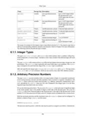


![Data TypesDepending on the front end to PostgreSQL you use, you might have additional work to do in terms ofescaping and unescaping bytea strings. For example, you might also have to escape line feeds andcarriage returns if your interface automatically translates these.8.5. Date/Time TypesPostgreSQL supports the full set of SQL date and time types, shown in Table 8.9. The operationsavailable on these data types are described in Section 9.9. Dates are counted according to the Gregoriancalendar, even in years before that calendar was introduced (see Section B.6 for more information).Table 8.9. Date/Time TypesName Storage Size Description Low Value High Value Resolutiontimestamp[ (p) ][ with-out timezone ]8 bytes both date andtime (no timezone)4713 BC 294276 AD 1 microsecondtimestamp[ (p) ]with timezone8 bytes both date andtime, with timezone4713 BC 294276 AD 1 microseconddate 4 bytes date (no timeof day)4713 BC 5874897 AD 1 daytime[ (p) ][ with-out timezone ]8 bytes time of day (nodate)00:00:00 24:00:00 1 microsecondtime[ (p) ]with timezone12 bytes time of day(no date), withtime zone00:00:00+1559 24:00:00-1559 1 microsecondinterval[ fields ][ (p) ]16 bytes time interval -178000000years178000000years1 microsecondNoteThe SQL standard requires that writing just timestamp be equivalent to timestampwithout time zone, and PostgreSQL honors that behavior. timestamptz is acceptedas an abbreviation for timestamp with time zone; this is a PostgreSQL extension.time, timestamp, and interval accept an optional precision value p which specifies the numberof fractional digits retained in the seconds field. By default, there is no explicit bound on precision.The allowed range of p is from 0 to 6.The interval type has an additional option, which is to restrict the set of stored fields by writingone of these phrases:YEARMONTH158](/image.pl?url=https%3a%2f%2fimage.slidesharecdn.com%2fpostgresql-16-a4-240621101854-e64a7806%2f85%2fpostgresql-16-3-latest-version-2024-25-pdf-196-638.jpg&f=jpg&w=240)
![Data TypesDAYHOURMINUTESECONDYEAR TO MONTHDAY TO HOURDAY TO MINUTEDAY TO SECONDHOUR TO MINUTEHOUR TO SECONDMINUTE TO SECONDNote that if both fields and p are specified, the fields must include SECOND, since the precisionapplies only to the seconds.The type time with time zone is defined by the SQL standard, but the definition exhibits prop-erties which lead to questionable usefulness. In most cases, a combination of date, time, time-stamp without time zone, and timestamp with time zone should provide a completerange of date/time functionality required by any application.8.5.1. Date/Time InputDate and time input is accepted in almost any reasonable format, including ISO 8601, SQL-compati-ble, traditional POSTGRES, and others. For some formats, ordering of day, month, and year in dateinput is ambiguous and there is support for specifying the expected ordering of these fields. Set theDateStyle parameter to MDY to select month-day-year interpretation, DMY to select day-month-yearinterpretation, or YMD to select year-month-day interpretation.PostgreSQL is more flexible in handling date/time input than the SQL standard requires. See Appen-dix B for the exact parsing rules of date/time input and for the recognized text fields including months,days of the week, and time zones.Remember that any date or time literal input needs to be enclosed in single quotes, like text strings.Refer to Section 4.1.2.7 for more information. SQL requires the following syntaxtype [ (p) ] 'value'where p is an optional precision specification giving the number of fractional digits in the secondsfield. Precision can be specified for time, timestamp, and interval types, and can range from0 to 6. If no precision is specified in a constant specification, it defaults to the precision of the literalvalue (but not more than 6 digits).8.5.1.1. DatesTable 8.10 shows some possible inputs for the date type.Table 8.10. Date InputExample Description1999-01-08 ISO 8601; January 8 in any mode (recommended format)January 8, 1999 unambiguous in any datestyle input mode1/8/1999 January 8 in MDY mode; August 1 in DMY mode1/18/1999 January 18 in MDY mode; rejected in other modes01/02/03 January 2, 2003 in MDY mode; February 1, 2003 in DMY mode;February 3, 2001 in YMD mode159](/image.pl?url=https%3a%2f%2fimage.slidesharecdn.com%2fpostgresql-16-a4-240621101854-e64a7806%2f85%2fpostgresql-16-3-latest-version-2024-25-pdf-197-638.jpg&f=jpg&w=240)
![Data TypesExample Description1999-Jan-08 January 8 in any modeJan-08-1999 January 8 in any mode08-Jan-1999 January 8 in any mode99-Jan-08 January 8 in YMD mode, else error08-Jan-99 January 8, except error in YMD modeJan-08-99 January 8, except error in YMD mode19990108 ISO 8601; January 8, 1999 in any mode990108 ISO 8601; January 8, 1999 in any mode1999.008 year and day of yearJ2451187 Julian dateJanuary 8, 99 BC year 99 BC8.5.1.2. TimesThe time-of-day types are time [ (p) ] without time zone and time [ (p) ] withtime zone. time alone is equivalent to time without time zone.Valid input for these types consists of a time of day followed by an optional time zone. (See Table 8.11and Table 8.12.) If a time zone is specified in the input for time without time zone, it is silentlyignored. You can also specify a date but it will be ignored, except when you use a time zone namethat involves a daylight-savings rule, such as America/New_York. In this case specifying the dateis required in order to determine whether standard or daylight-savings time applies. The appropriatetime zone offset is recorded in the time with time zone value and is output as stored; it isnot adjusted to the active time zone.Table 8.11. Time InputExample Description04:05:06.789 ISO 860104:05:06 ISO 860104:05 ISO 8601040506 ISO 860104:05 AM same as 04:05; AM does not affectvalue04:05 PM same as 16:05; input hour must be <=1204:05:06.789-8 ISO 8601, with time zone as UTC off-set04:05:06-08:00 ISO 8601, with time zone as UTC off-set04:05-08:00 ISO 8601, with time zone as UTC off-set040506-08 ISO 8601, with time zone as UTC off-set040506+0730 ISO 8601, with fractional-hour timezone as UTC offset040506+07:30:00 UTC offset specified to seconds (notallowed in ISO 8601)160](/image.pl?url=https%3a%2f%2fimage.slidesharecdn.com%2fpostgresql-16-a4-240621101854-e64a7806%2f85%2fpostgresql-16-3-latest-version-2024-25-pdf-198-638.jpg&f=jpg&w=240)


![Data Typesmost recently meant) on the specified date; but, as with the EST example above, this is not necessarilythe same as local civil time on that date.In all cases, timezone names and abbreviations are recognized case-insensitively. (This is a changefrom PostgreSQL versions prior to 8.2, which were case-sensitive in some contexts but not others.)Neither timezone names nor abbreviations are hard-wired into the server; they are obtained from con-figuration files stored under .../share/timezone/ and .../share/timezonesets/ ofthe installation directory (see Section B.4).The TimeZone configuration parameter can be set in the file postgresql.conf, or in any of theother standard ways described in Chapter 20. There are also some special ways to set it:• The SQL command SET TIME ZONE sets the time zone for the session. This is an alternativespelling of SET TIMEZONE TO with a more SQL-spec-compatible syntax.• The PGTZ environment variable is used by libpq clients to send a SET TIME ZONE commandto the server upon connection.8.5.4. Interval Inputinterval values can be written using the following verbose syntax:[@] quantity unit [quantity unit...] [direction]where quantity is a number (possibly signed); unit is microsecond, millisecond, sec-ond, minute, hour, day, week, month, year, decade, century, millennium, or abbrevi-ations or plurals of these units; direction can be ago or empty. The at sign (@) is optional noise.The amounts of the different units are implicitly added with appropriate sign accounting. ago negatesall the fields. This syntax is also used for interval output, if IntervalStyle is set to postgres_ver-bose.Quantities of days, hours, minutes, and seconds can be specified without explicit unit markings. Forexample, '1 12:59:10' is read the same as '1 day 12 hours 59 min 10 sec'. Also,a combination of years and months can be specified with a dash; for example '200-10' is read thesame as '200 years 10 months'. (These shorter forms are in fact the only ones allowed by theSQL standard, and are used for output when IntervalStyle is set to sql_standard.)Interval values can also be written as ISO 8601 time intervals, using either the “format with designa-tors” of the standard's section 4.4.3.2 or the “alternative format” of section 4.4.3.3. The format withdesignators looks like this:P quantity unit [ quantity unit ...] [ T [ quantity unit ...]]The string must start with a P, and may include a T that introduces the time-of-day units. The availableunit abbreviations are given in Table 8.16. Units may be omitted, and may be specified in any order,but units smaller than a day must appear after T. In particular, the meaning of M depends on whetherit is before or after T.Table 8.16. ISO 8601 Interval Unit AbbreviationsAbbreviation MeaningY YearsM Months (in the date part)W WeeksD Days165](/image.pl?url=https%3a%2f%2fimage.slidesharecdn.com%2fpostgresql-16-a4-240621101854-e64a7806%2f85%2fpostgresql-16-3-latest-version-2024-25-pdf-203-638.jpg&f=jpg&w=240)
![Data TypesAbbreviation MeaningH HoursM Minutes (in the time part)S SecondsIn the alternative format:P [ years-months-days ] [ T hours:minutes:seconds ]the string must begin with P, and a T separates the date and time parts of the interval. The values aregiven as numbers similar to ISO 8601 dates.When writing an interval constant with a fields specification, or when assigning a string to an in-terval column that was defined with a fields specification, the interpretation of unmarked quantitiesdepends on the fields. For example INTERVAL '1' YEAR is read as 1 year, whereas INTER-VAL '1' means 1 second. Also, field values “to the right” of the least significant field allowed by thefields specification are silently discarded. For example, writing INTERVAL '1 day 2:03:04'HOUR TO MINUTE results in dropping the seconds field, but not the day field.According to the SQL standard all fields of an interval value must have the same sign, so a leadingnegative sign applies to all fields; for example the negative sign in the interval literal '-1 2:03:04'applies to both the days and hour/minute/second parts. PostgreSQL allows the fields to have differentsigns, and traditionally treats each field in the textual representation as independently signed, so thatthe hour/minute/second part is considered positive in this example. If IntervalStyle is set tosql_standard then a leading sign is considered to apply to all fields (but only if no additionalsigns appear). Otherwise the traditional PostgreSQL interpretation is used. To avoid ambiguity, it'srecommended to attach an explicit sign to each field if any field is negative.Internally, interval values are stored as three integral fields: months, days, and microseconds.These fields are kept separate because the number of days in a month varies, while a day can have 23 or25 hours if a daylight savings time transition is involved. An interval input string that uses other unitsis normalized into this format, and then reconstructed in a standardized way for output, for example:SELECT '2 years 15 months 100 weeks 99 hours 123456789milliseconds'::interval;interval---------------------------------------3 years 3 mons 700 days 133:17:36.789Here weeks, which are understood as “7 days”, have been kept separate, while the smaller and largertime units were combined and normalized.Input field values can have fractional parts, for example '1.5 weeks' or '01:02:03.45'. How-ever, because interval internally stores only integral fields, fractional values must be convertedinto smaller units. Fractional parts of units greater than months are rounded to be an integer numberof months, e.g. '1.5 years' becomes '1 year 6 mons'. Fractional parts of weeks and daysare computed to be an integer number of days and microseconds, assuming 30 days per month and24 hours per day, e.g., '1.75 months' becomes 1 mon 22 days 12:00:00. Only secondswill ever be shown as fractional on output.Table 8.17 shows some examples of valid interval input.Table 8.17. Interval InputExample Description1-2 SQL standard format: 1 year 2 months166](/image.pl?url=https%3a%2f%2fimage.slidesharecdn.com%2fpostgresql-16-a4-240621101854-e64a7806%2f85%2fpostgresql-16-3-latest-version-2024-25-pdf-204-638.jpg&f=jpg&w=240)


![Data TypesName Storage Size Description Representationpath 16+16n bytes Open path [(x1,y1),...]polygon 40+16n bytes Polygon (similar to closed path) ((x1,y1),...)circle 24 bytes Circle <(x,y),r> (centerpoint and radius)A rich set of functions and operators is available to perform various geometric operations such asscaling, translation, rotation, and determining intersections. They are explained in Section 9.11.8.8.1. PointsPoints are the fundamental two-dimensional building block for geometric types. Values of type pointare specified using either of the following syntaxes:( x , y )x , ywhere x and y are the respective coordinates, as floating-point numbers.Points are output using the first syntax.8.8.2. LinesLines are represented by the linear equation Ax + By + C = 0, where A and B are not both zero. Valuesof type line are input and output in the following form:{ A, B, C }Alternatively, any of the following forms can be used for input:[ ( x1 , y1 ) , ( x2 , y2 ) ]( ( x1 , y1 ) , ( x2 , y2 ) )( x1 , y1 ) , ( x2 , y2 )x1 , y1 , x2 , y2where (x1,y1) and (x2,y2) are two different points on the line.8.8.3. Line SegmentsLine segments are represented by pairs of points that are the endpoints of the segment. Values of typelseg are specified using any of the following syntaxes:[ ( x1 , y1 ) , ( x2 , y2 ) ]( ( x1 , y1 ) , ( x2 , y2 ) )( x1 , y1 ) , ( x2 , y2 )x1 , y1 , x2 , y2where (x1,y1) and (x2,y2) are the end points of the line segment.Line segments are output using the first syntax.8.8.4. Boxes171](/image.pl?url=https%3a%2f%2fimage.slidesharecdn.com%2fpostgresql-16-a4-240621101854-e64a7806%2f85%2fpostgresql-16-3-latest-version-2024-25-pdf-209-638.jpg&f=jpg&w=240)
 , ... , ( xn , yn ) )( x1 , y1 ) , ... , ( xn , yn )( x1 , y1 , ... , xn , yn )x1 , y1 , ... , xn , ynwhere the points are the end points of the line segments comprising the path. Square brackets ([])indicate an open path, while parentheses (()) indicate a closed path. When the outermost parenthesesare omitted, as in the third through fifth syntaxes, a closed path is assumed.Paths are output using the first or second syntax, as appropriate.8.8.6. PolygonsPolygons are represented by lists of points (the vertexes of the polygon). Polygons are very similarto closed paths; the essential difference is that a polygon is considered to include the area within it,while a path is not.Values of type polygon are specified using any of the following syntaxes:( ( x1 , y1 ) , ... , ( xn , yn ) )( x1 , y1 ) , ... , ( xn , yn )( x1 , y1 , ... , xn , yn )x1 , y1 , ... , xn , ynwhere the points are the end points of the line segments comprising the boundary of the polygon.Polygons are output using the first syntax.8.8.7. CirclesCircles are represented by a center point and radius. Values of type circle are specified using anyof the following syntaxes:< ( x , y ) , r >172](/image.pl?url=https%3a%2f%2fimage.slidesharecdn.com%2fpostgresql-16-a4-240621101854-e64a7806%2f85%2fpostgresql-16-3-latest-version-2024-25-pdf-210-638.jpg&f=jpg&w=240)


![Data TypesXMLPARSE ( { DOCUMENT | CONTENT } value)Examples:XMLPARSE (DOCUMENT '<?xml version="1.0"?><book><title>Manual</title><chapter>...</chapter></book>')XMLPARSE (CONTENT 'abc<foo>bar</foo><bar>foo</bar>')While this is the only way to convert character strings into XML values according to the SQL standard,the PostgreSQL-specific syntaxes:xml '<foo>bar</foo>''<foo>bar</foo>'::xmlcan also be used.The xml type does not validate input values against a document type declaration (DTD), even whenthe input value specifies a DTD. There is also currently no built-in support for validating against otherXML schema languages such as XML Schema.The inverse operation, producing a character string value from xml, uses the function xmlserial-ize:XMLSERIALIZE ( { DOCUMENT | CONTENT } value AS type [ [ NO ]INDENT ] )type can be character, character varying, or text (or an alias for one of those). Again,according to the SQL standard, this is the only way to convert between type xml and character types,but PostgreSQL also allows you to simply cast the value.The INDENT option causes the result to be pretty-printed, while NO INDENT (which is the default)just emits the original input string. Casting to a character type likewise produces the original string.When a character string value is cast to or from type xml without going through XMLPARSE or XM-LSERIALIZE, respectively, the choice of DOCUMENT versus CONTENT is determined by the “XMLoption” session configuration parameter, which can be set using the standard command:SET XML OPTION { DOCUMENT | CONTENT };or the more PostgreSQL-like syntaxSET xmloption TO { DOCUMENT | CONTENT };The default is CONTENT, so all forms of XML data are allowed.8.13.2. Encoding HandlingCare must be taken when dealing with multiple character encodings on the client, server, and in theXML data passed through them. When using the text mode to pass queries to the server and queryresults to the client (which is the normal mode), PostgreSQL converts all character data passed be-tween the client and the server and vice versa to the character encoding of the respective end; seeSection 24.3. This includes string representations of XML values, such as in the above examples. Thiswould ordinarily mean that encoding declarations contained in XML data can become invalid as thecharacter data is converted to other encodings while traveling between client and server, because theembedded encoding declaration is not changed. To cope with this behavior, encoding declarationscontained in character strings presented for input to the xml type are ignored, and content is assumed180](/image.pl?url=https%3a%2f%2fimage.slidesharecdn.com%2fpostgresql-16-a4-240621101854-e64a7806%2f85%2fpostgresql-16-3-latest-version-2024-25-pdf-218-638.jpg&f=jpg&w=240)


![Data TypesJSON primitive type PostgreSQL type Notesnumber numeric NaN and infinity values are disallowedboolean boolean Only lowercase true and false spellings areacceptednull (none) SQL NULL is a different concept8.14.1. JSON Input and Output SyntaxThe input/output syntax for the JSON data types is as specified in RFC 7159.The following are all valid json (or jsonb) expressions:-- Simple scalar/primitive value-- Primitive values can be numbers, quoted strings, true, false, ornullSELECT '5'::json;-- Array of zero or more elements (elements need not be of sametype)SELECT '[1, 2, "foo", null]'::json;-- Object containing pairs of keys and values-- Note that object keys must always be quoted stringsSELECT '{"bar": "baz", "balance": 7.77, "active": false}'::json;-- Arrays and objects can be nested arbitrarilySELECT '{"foo": [true, "bar"], "tags": {"a": 1, "b": null}}'::json;As previously stated, when a JSON value is input and then printed without any additional processing,json outputs the same text that was input, while jsonb does not preserve semantically-insignificantdetails such as whitespace. For example, note the differences here:SELECT '{"bar": "baz", "balance": 7.77, "active":false}'::json;json-------------------------------------------------{"bar": "baz", "balance": 7.77, "active":false}(1 row)SELECT '{"bar": "baz", "balance": 7.77, "active":false}'::jsonb;jsonb--------------------------------------------------{"bar": "baz", "active": false, "balance": 7.77}(1 row)One semantically-insignificant detail worth noting is that in jsonb, numbers will be printed accordingto the behavior of the underlying numeric type. In practice this means that numbers entered with Enotation will be printed without it, for example:SELECT '{"reading": 1.230e-5}'::json, '{"reading":1.230e-5}'::jsonb;json | jsonb-----------------------+-------------------------{"reading": 1.230e-5} | {"reading": 0.00001230}(1 row)183](/image.pl?url=https%3a%2f%2fimage.slidesharecdn.com%2fpostgresql-16-a4-240621101854-e64a7806%2f85%2fpostgresql-16-3-latest-version-2024-25-pdf-221-638.jpg&f=jpg&w=240)
![Data TypesHowever, jsonb will preserve trailing fractional zeroes, as seen in this example, even though thoseare semantically insignificant for purposes such as equality checks.For the list of built-in functions and operators available for constructing and processing JSON values,see Section 9.16.8.14.2. Designing JSON DocumentsRepresenting data as JSON can be considerably more flexible than the traditional relational data mod-el, which is compelling in environments where requirements are fluid. It is quite possible for bothapproaches to co-exist and complement each other within the same application. However, even forapplications where maximal flexibility is desired, it is still recommended that JSON documents havea somewhat fixed structure. The structure is typically unenforced (though enforcing some businessrules declaratively is possible), but having a predictable structure makes it easier to write queries thatusefully summarize a set of “documents” (datums) in a table.JSON data is subject to the same concurrency-control considerations as any other data type whenstored in a table. Although storing large documents is practicable, keep in mind that any update ac-quires a row-level lock on the whole row. Consider limiting JSON documents to a manageable sizein order to decrease lock contention among updating transactions. Ideally, JSON documents shouldeach represent an atomic datum that business rules dictate cannot reasonably be further subdividedinto smaller datums that could be modified independently.8.14.3. jsonb Containment and ExistenceTesting containment is an important capability of jsonb. There is no parallel set of facilities for thejson type. Containment tests whether one jsonb document has contained within it another one.These examples return true except as noted:-- Simple scalar/primitive values contain only the identical value:SELECT '"foo"'::jsonb @> '"foo"'::jsonb;-- The array on the right side is contained within the one on theleft:SELECT '[1, 2, 3]'::jsonb @> '[1, 3]'::jsonb;-- Order of array elements is not significant, so this is alsotrue:SELECT '[1, 2, 3]'::jsonb @> '[3, 1]'::jsonb;-- Duplicate array elements don't matter either:SELECT '[1, 2, 3]'::jsonb @> '[1, 2, 2]'::jsonb;-- The object with a single pair on the right side is contained-- within the object on the left side:SELECT '{"product": "PostgreSQL", "version": 9.4, "jsonb":true}'::jsonb @> '{"version": 9.4}'::jsonb;-- The array on the right side is not considered contained withinthe-- array on the left, even though a similar array is nested withinit:SELECT '[1, 2, [1, 3]]'::jsonb @> '[1, 3]'::jsonb; -- yields false-- But with a layer of nesting, it is contained:SELECT '[1, 2, [1, 3]]'::jsonb @> '[[1, 3]]'::jsonb;184](/image.pl?url=https%3a%2f%2fimage.slidesharecdn.com%2fpostgresql-16-a4-240621101854-e64a7806%2f85%2fpostgresql-16-3-latest-version-2024-25-pdf-222-638.jpg&f=jpg&w=240)
![Data Types-- Similarly, containment is not reported here:SELECT '{"foo": {"bar": "baz"}}'::jsonb @> '{"bar": "baz"}'::jsonb;-- yields false-- A top-level key and an empty object is contained:SELECT '{"foo": {"bar": "baz"}}'::jsonb @> '{"foo": {}}'::jsonb;The general principle is that the contained object must match the containing object as to structure anddata contents, possibly after discarding some non-matching array elements or object key/value pairsfrom the containing object. But remember that the order of array elements is not significant whendoing a containment match, and duplicate array elements are effectively considered only once.As a special exception to the general principle that the structures must match, an array may containa primitive value:-- This array contains the primitive string value:SELECT '["foo", "bar"]'::jsonb @> '"bar"'::jsonb;-- This exception is not reciprocal -- non-containment is reportedhere:SELECT '"bar"'::jsonb @> '["bar"]'::jsonb; -- yields falsejsonb also has an existence operator, which is a variation on the theme of containment: it testswhether a string (given as a text value) appears as an object key or array element at the top level ofthe jsonb value. These examples return true except as noted:-- String exists as array element:SELECT '["foo", "bar", "baz"]'::jsonb ? 'bar';-- String exists as object key:SELECT '{"foo": "bar"}'::jsonb ? 'foo';-- Object values are not considered:SELECT '{"foo": "bar"}'::jsonb ? 'bar'; -- yields false-- As with containment, existence must match at the top level:SELECT '{"foo": {"bar": "baz"}}'::jsonb ? 'bar'; -- yields false-- A string is considered to exist if it matches a primitive JSONstring:SELECT '"foo"'::jsonb ? 'foo';JSON objects are better suited than arrays for testing containment or existence when there are manykeys or elements involved, because unlike arrays they are internally optimized for searching, and donot need to be searched linearly.TipBecause JSON containment is nested, an appropriate query can skip explicit selection of sub-objects. As an example, suppose that we have a doc column containing objects at the top level,with most objects containing tags fields that contain arrays of sub-objects. This query findsentries in which sub-objects containing both "term":"paris" and "term":"food" ap-pear, while ignoring any such keys outside the tags array:SELECT doc->'site_name' FROM websitesWHERE doc @> '{"tags":[{"term":"paris"}, {"term":"food"}]}';185](/image.pl?url=https%3a%2f%2fimage.slidesharecdn.com%2fpostgresql-16-a4-240621101854-e64a7806%2f85%2fpostgresql-16-3-latest-version-2024-25-pdf-223-638.jpg&f=jpg&w=240)
![Data TypesOne could accomplish the same thing with, say,SELECT doc->'site_name' FROM websitesWHERE doc->'tags' @> '[{"term":"paris"}, {"term":"food"}]';but that approach is less flexible, and often less efficient as well.On the other hand, the JSON existence operator is not nested: it will only look for the specifiedkey or array element at top level of the JSON value.The various containment and existence operators, along with all other JSON operators and functionsare documented in Section 9.16.8.14.4. jsonb IndexingGIN indexes can be used to efficiently search for keys or key/value pairs occurring within a largenumber of jsonb documents (datums). Two GIN “operator classes” are provided, offering differentperformance and flexibility trade-offs.The default GIN operator class for jsonb supports queries with the key-exists operators ?, ?| and?&, the containment operator @>, and the jsonpath match operators @? and @@. (For details of thesemantics that these operators implement, see Table 9.46.) An example of creating an index with thisoperator class is:CREATE INDEX idxgin ON api USING GIN (jdoc);The non-default GIN operator class jsonb_path_ops does not support the key-exists operators,but it does support @>, @? and @@. An example of creating an index with this operator class is:CREATE INDEX idxginp ON api USING GIN (jdoc jsonb_path_ops);Consider the example of a table that stores JSON documents retrieved from a third-party web service,with a documented schema definition. A typical document is:{"guid": "9c36adc1-7fb5-4d5b-83b4-90356a46061a","name": "Angela Barton","is_active": true,"company": "Magnafone","address": "178 Howard Place, Gulf, Washington, 702","registered": "2009-11-07T08:53:22 +08:00","latitude": 19.793713,"longitude": 86.513373,"tags": ["enim","aliquip","qui"]}We store these documents in a table named api, in a jsonb column named jdoc. If a GIN index iscreated on this column, queries like the following can make use of the index:-- Find documents in which the key "company" has value "Magnafone"186](/image.pl?url=https%3a%2f%2fimage.slidesharecdn.com%2fpostgresql-16-a4-240621101854-e64a7806%2f85%2fpostgresql-16-3-latest-version-2024-25-pdf-224-638.jpg&f=jpg&w=240)
![Data TypesSELECT jdoc->'guid', jdoc->'name' FROM api WHERE jdoc @>'{"company": "Magnafone"}';However, the index could not be used for queries like the following, because though the operator ? isindexable, it is not applied directly to the indexed column jdoc:-- Find documents in which the key "tags" contains key or arrayelement "qui"SELECT jdoc->'guid', jdoc->'name' FROM api WHERE jdoc -> 'tags' ?'qui';Still, with appropriate use of expression indexes, the above query can use an index. If querying forparticular items within the "tags" key is common, defining an index like this may be worthwhile:CREATE INDEX idxgintags ON api USING GIN ((jdoc -> 'tags'));Now, the WHERE clause jdoc -> 'tags' ? 'qui' will be recognized as an application of theindexable operator ? to the indexed expression jdoc -> 'tags'. (More information on expressionindexes can be found in Section 11.7.)Another approach to querying is to exploit containment, for example:-- Find documents in which the key "tags" contains array element"qui"SELECT jdoc->'guid', jdoc->'name' FROM api WHERE jdoc @> '{"tags":["qui"]}';A simple GIN index on the jdoc column can support this query. But note that such an index willstore copies of every key and value in the jdoc column, whereas the expression index of the previousexample stores only data found under the tags key. While the simple-index approach is far moreflexible (since it supports queries about any key), targeted expression indexes are likely to be smallerand faster to search than a simple index.GIN indexes also support the @? and @@ operators, which perform jsonpath matching. ExamplesareSELECT jdoc->'guid', jdoc->'name' FROM api WHERE jdoc @?'$.tags[*] ? (@ == "qui")';SELECT jdoc->'guid', jdoc->'name' FROM api WHERE jdoc @@ '$.tags[*]== "qui"';For these operators, a GIN index extracts clauses of the form accessors_chain = constantout of the jsonpath pattern, and does the index search based on the keys and values mentionedin these clauses. The accessors chain may include .key, [*], and [index] accessors. The json-b_ops operator class also supports .* and .** accessors, but the jsonb_path_ops operator classdoes not.Although the jsonb_path_ops operator class supports only queries with the @>, @? and @@ oper-ators, it has notable performance advantages over the default operator class jsonb_ops. A json-b_path_ops index is usually much smaller than a jsonb_ops index over the same data, and thespecificity of searches is better, particularly when queries contain keys that appear frequently in thedata. Therefore search operations typically perform better than with the default operator class.The technical difference between a jsonb_ops and a jsonb_path_ops GIN index is that theformer creates independent index items for each key and value in the data, while the latter creates187](/image.pl?url=https%3a%2f%2fimage.slidesharecdn.com%2fpostgresql-16-a4-240621101854-e64a7806%2f85%2fpostgresql-16-3-latest-version-2024-25-pdf-225-638.jpg&f=jpg&w=240)
![Data Typesindex items only for each value in the data. 5Basically, each jsonb_path_ops index item is ahash of the value and the key(s) leading to it; for example to index {"foo": {"bar": "baz"}},a single index item would be created incorporating all three of foo, bar, and baz into the hashvalue. Thus a containment query looking for this structure would result in an extremely specific indexsearch; but there is no way at all to find out whether foo appears as a key. On the other hand, ajsonb_ops index would create three index items representing foo, bar, and baz separately; thento do the containment query, it would look for rows containing all three of these items. While GINindexes can perform such an AND search fairly efficiently, it will still be less specific and slowerthan the equivalent jsonb_path_ops search, especially if there are a very large number of rowscontaining any single one of the three index items.A disadvantage of the jsonb_path_ops approach is that it produces no index entries for JSONstructures not containing any values, such as {"a": {}}. If a search for documents containing sucha structure is requested, it will require a full-index scan, which is quite slow. jsonb_path_ops istherefore ill-suited for applications that often perform such searches.jsonb also supports btree and hash indexes. These are usually useful only if it's important tocheck equality of complete JSON documents. The btree ordering for jsonb datums is seldom ofgreat interest, but for completeness it is:Object > Array > Boolean > Number > String > NullObject with n pairs > object with n - 1 pairsArray with n elements > array with n - 1 elementsObjects with equal numbers of pairs are compared in the order:key-1, value-1, key-2 ...Note that object keys are compared in their storage order; in particular, since shorter keys are storedbefore longer keys, this can lead to results that might be unintuitive, such as:{ "aa": 1, "c": 1} > {"b": 1, "d": 1}Similarly, arrays with equal numbers of elements are compared in the order:element-1, element-2 ...Primitive JSON values are compared using the same comparison rules as for the underlying Post-greSQL data type. Strings are compared using the default database collation.8.14.5. jsonb SubscriptingThe jsonb data type supports array-style subscripting expressions to extract and modify elements.Nested values can be indicated by chaining subscripting expressions, following the same rules as thepath argument in the jsonb_set function. If a jsonb value is an array, numeric subscripts startat zero, and negative integers count backwards from the last element of the array. Slice expressionsare not supported. The result of a subscripting expression is always of the jsonb data type.UPDATE statements may use subscripting in the SET clause to modify jsonb values. Subscript pathsmust be traversable for all affected values insofar as they exist. For instance, the path val['a']['b']['c'] can be traversed all the way to c if every val, val['a'], and val['a']['b']5For this purpose, the term “value” includes array elements, though JSON terminology sometimes considers array elements distinct fromvalues within objects.188](/image.pl?url=https%3a%2f%2fimage.slidesharecdn.com%2fpostgresql-16-a4-240621101854-e64a7806%2f85%2fpostgresql-16-3-latest-version-2024-25-pdf-226-638.jpg&f=jpg&w=240)
![Data Typesis an object. If any val['a'] or val['a']['b'] is not defined, it will be created as an emptyobject and filled as necessary. However, if any val itself or one of the intermediary values is definedas a non-object such as a string, number, or jsonb null, traversal cannot proceed so an error israised and the transaction aborted.An example of subscripting syntax:-- Extract object value by keySELECT ('{"a": 1}'::jsonb)['a'];-- Extract nested object value by key pathSELECT ('{"a": {"b": {"c": 1}}}'::jsonb)['a']['b']['c'];-- Extract array element by indexSELECT ('[1, "2", null]'::jsonb)[1];-- Update object value by key. Note the quotes around '1': theassigned-- value must be of the jsonb type as wellUPDATE table_name SET jsonb_field['key'] = '1';-- This will raise an error if any record's jsonb_field['a']['b']is something-- other than an object. For example, the value {"a": 1} has anumeric value-- of the key 'a'.UPDATE table_name SET jsonb_field['a']['b']['c'] = '1';-- Filter records using a WHERE clause with subscripting. Since theresult of-- subscripting is jsonb, the value we compare it against must alsobe jsonb.-- The double quotes make "value" also a valid jsonb string.SELECT * FROM table_name WHERE jsonb_field['key'] = '"value"';jsonb assignment via subscripting handles a few edge cases differently from jsonb_set. When asource jsonb value is NULL, assignment via subscripting will proceed as if it was an empty JSONvalue of the type (object or array) implied by the subscript key:-- Where jsonb_field was NULL, it is now {"a": 1}UPDATE table_name SET jsonb_field['a'] = '1';-- Where jsonb_field was NULL, it is now [1]UPDATE table_name SET jsonb_field[0] = '1';If an index is specified for an array containing too few elements, NULL elements will be appendeduntil the index is reachable and the value can be set.-- Where jsonb_field was [], it is now [null, null, 2];-- where jsonb_field was [0], it is now [0, null, 2]UPDATE table_name SET jsonb_field[2] = '2';A jsonb value will accept assignments to nonexistent subscript paths as long as the last existingelement to be traversed is an object or array, as implied by the corresponding subscript (the elementindicated by the last subscript in the path is not traversed and may be anything). Nested array and189](/image.pl?url=https%3a%2f%2fimage.slidesharecdn.com%2fpostgresql-16-a4-240621101854-e64a7806%2f85%2fpostgresql-16-3-latest-version-2024-25-pdf-227-638.jpg&f=jpg&w=240)
![Data Typesobject structures will be created, and in the former case null-padded, as specified by the subscriptpath until the assigned value can be placed.-- Where jsonb_field was {}, it is now {"a": [{"b": 1}]}UPDATE table_name SET jsonb_field['a'][0]['b'] = '1';-- Where jsonb_field was [], it is now [null, {"a": 1}]UPDATE table_name SET jsonb_field[1]['a'] = '1';8.14.6. TransformsAdditional extensions are available that implement transforms for the jsonb type for different pro-cedural languages.The extensions for PL/Perl are called jsonb_plperl and jsonb_plperlu. If you use them,jsonb values are mapped to Perl arrays, hashes, and scalars, as appropriate.The extension for PL/Python is called jsonb_plpython3u. If you use it, jsonb values are mappedto Python dictionaries, lists, and scalars, as appropriate.Of these extensions, jsonb_plperl is considered “trusted”, that is, it can be installed by non-superusers who have CREATE privilege on the current database. The rest require superuser privilegeto install.8.14.7. jsonpath TypeThe jsonpath type implements support for the SQL/JSON path language in PostgreSQL to effi-ciently query JSON data. It provides a binary representation of the parsed SQL/JSON path expressionthat specifies the items to be retrieved by the path engine from the JSON data for further processingwith the SQL/JSON query functions.The semantics of SQL/JSON path predicates and operators generally follow SQL. At the same time,to provide a natural way of working with JSON data, SQL/JSON path syntax uses some JavaScriptconventions:• Dot (.) is used for member access.• Square brackets ([]) are used for array access.• SQL/JSON arrays are 0-relative, unlike regular SQL arrays that start from 1.Numeric literals in SQL/JSON path expressions follow JavaScript rules, which are different from bothSQL and JSON in some minor details. For example, SQL/JSON path allows .1 and 1., which areinvalid in JSON. Non-decimal integer literals and underscore separators are supported, for example,1_000_000, 0x1EEE_FFFF, 0o273, 0b100101. In SQL/JSON path (and in JavaScript, but notin SQL proper), there must not be an underscore separator directly after the radix prefix.An SQL/JSON path expression is typically written in an SQL query as an SQL character string literal,so it must be enclosed in single quotes, and any single quotes desired within the value must be doubled(see Section 4.1.2.1). Some forms of path expressions require string literals within them. These em-bedded string literals follow JavaScript/ECMAScript conventions: they must be surrounded by doublequotes, and backslash escapes may be used within them to represent otherwise-hard-to-type charac-ters. In particular, the way to write a double quote within an embedded string literal is ", and to writea backslash itself, you must write . Other special backslash sequences include those recognized inJavaScript strings: b, f, n, r, t, v for various ASCII control characters, xNN for a charactercode written with only two hex digits, uNNNN for a Unicode character identified by its 4-hex-digitcode point, and u{N...} for a Unicode character code point written with 1 to 6 hex digits.A path expression consists of a sequence of path elements, which can be any of the following:190](/image.pl?url=https%3a%2f%2fimage.slidesharecdn.com%2fpostgresql-16-a4-240621101854-e64a7806%2f85%2fpostgresql-16-3-latest-version-2024-25-pdf-228-638.jpg&f=jpg&w=240)
![Data Types• Path literals of JSON primitive types: Unicode text, numeric, true, false, or null.• Path variables listed in Table 8.24.• Accessor operators listed in Table 8.25.• jsonpath operators and methods listed in Section 9.16.2.2.• Parentheses, which can be used to provide filter expressions or define the order of path evaluation.For details on using jsonpath expressions with SQL/JSON query functions, see Section 9.16.2.Table 8.24. jsonpath VariablesVariable Description$ A variable representing the JSON value being queried (the con-text item).$varname A named variable. Its value can be set by the parameter vars ofseveral JSON processing functions; see Table 9.49 for details.@ A variable representing the result of path evaluation in filter ex-pressions.Table 8.25. jsonpath AccessorsAccessor Operator Description.key."$varname"Member accessor that returns an object member with the speci-fied key. If the key name matches some named variable startingwith $ or does not meet the JavaScript rules for an identifier, itmust be enclosed in double quotes to make it a string literal..* Wildcard member accessor that returns the values of all memberslocated at the top level of the current object..** Recursive wildcard member accessor that processes all levels ofthe JSON hierarchy of the current object and returns all the mem-ber values, regardless of their nesting level. This is a PostgreSQLextension of the SQL/JSON standard..**{level}.**{start_level toend_level}Like .**, but selects only the specified levels of the JSON hier-archy. Nesting levels are specified as integers. Level zero corre-sponds to the current object. To access the lowest nesting level,you can use the last keyword. This is a PostgreSQL extensionof the SQL/JSON standard.[subscript, ...] Array element accessor. subscript can be given in two forms:index or start_index to end_index. The first form re-turns a single array element by its index. The second form returnsan array slice by the range of indexes, including the elements thatcorrespond to the provided start_index and end_index.The specified index can be an integer, as well as an expressionreturning a single numeric value, which is automatically cast tointeger. Index zero corresponds to the first array element. Youcan also use the last keyword to denote the last array element,which is useful for handling arrays of unknown length.[*] Wildcard array element accessor that returns all array elements.8.15. Arrays191](/image.pl?url=https%3a%2f%2fimage.slidesharecdn.com%2fpostgresql-16-a4-240621101854-e64a7806%2f85%2fpostgresql-16-3-latest-version-2024-25-pdf-229-638.jpg&f=jpg&w=240)
![Data TypesPostgreSQL allows columns of a table to be defined as variable-length multidimensional arrays. Arraysof any built-in or user-defined base type, enum type, composite type, range type, or domain can becreated.8.15.1. Declaration of Array TypesTo illustrate the use of array types, we create this table:CREATE TABLE sal_emp (name text,pay_by_quarter integer[],schedule text[][]);As shown, an array data type is named by appending square brackets ([]) to the data type name ofthe array elements. The above command will create a table named sal_emp with a column of typetext (name), a one-dimensional array of type integer (pay_by_quarter), which representsthe employee's salary by quarter, and a two-dimensional array of text (schedule), which repre-sents the employee's weekly schedule.The syntax for CREATE TABLE allows the exact size of arrays to be specified, for example:CREATE TABLE tictactoe (squares integer[3][3]);However, the current implementation ignores any supplied array size limits, i.e., the behavior is thesame as for arrays of unspecified length.The current implementation does not enforce the declared number of dimensions either. Arrays ofa particular element type are all considered to be of the same type, regardless of size or number ofdimensions. So, declaring the array size or number of dimensions in CREATE TABLE is simplydocumentation; it does not affect run-time behavior.An alternative syntax, which conforms to the SQL standard by using the keyword ARRAY, can be usedfor one-dimensional arrays. pay_by_quarter could have been defined as:pay_by_quarter integer ARRAY[4],Or, if no array size is to be specified:pay_by_quarter integer ARRAY,As before, however, PostgreSQL does not enforce the size restriction in any case.8.15.2. Array Value InputTo write an array value as a literal constant, enclose the element values within curly braces and separatethem by commas. (If you know C, this is not unlike the C syntax for initializing structures.) You canput double quotes around any element value, and must do so if it contains commas or curly braces.(More details appear below.) Thus, the general format of an array constant is the following:'{ val1 delim val2 delim ... }'192](/image.pl?url=https%3a%2f%2fimage.slidesharecdn.com%2fpostgresql-16-a4-240621101854-e64a7806%2f85%2fpostgresql-16-3-latest-version-2024-25-pdf-230-638.jpg&f=jpg&w=240)

![Data TypesARRAY[10000, 10000, 10000, 10000],ARRAY[['meeting', 'lunch'], ['training', 'presentation']]);INSERT INTO sal_empVALUES ('Carol',ARRAY[20000, 25000, 25000, 25000],ARRAY[['breakfast', 'consulting'], ['meeting', 'lunch']]);Notice that the array elements are ordinary SQL constants or expressions; for instance, string literalsare single quoted, instead of double quoted as they would be in an array literal. The ARRAY constructorsyntax is discussed in more detail in Section 4.2.12.8.15.3. Accessing ArraysNow, we can run some queries on the table. First, we show how to access a single element of an array.This query retrieves the names of the employees whose pay changed in the second quarter:SELECT name FROM sal_emp WHERE pay_by_quarter[1] <>pay_by_quarter[2];name-------Carol(1 row)The array subscript numbers are written within square brackets. By default PostgreSQL uses a one-based numbering convention for arrays, that is, an array of n elements starts with array[1] andends with array[n].This query retrieves the third quarter pay of all employees:SELECT pay_by_quarter[3] FROM sal_emp;pay_by_quarter----------------1000025000(2 rows)We can also access arbitrary rectangular slices of an array, or subarrays. An array slice is denoted bywriting lower-bound:upper-bound for one or more array dimensions. For example, this queryretrieves the first item on Bill's schedule for the first two days of the week:SELECT schedule[1:2][1:1] FROM sal_emp WHERE name = 'Bill';schedule------------------------{{meeting},{training}}(1 row)If any dimension is written as a slice, i.e., contains a colon, then all dimensions are treated as slices.Any dimension that has only a single number (no colon) is treated as being from 1 to the numberspecified. For example, [2] is treated as [1:2], as in this example:SELECT schedule[1:2][2] FROM sal_emp WHERE name = 'Bill';194](/image.pl?url=https%3a%2f%2fimage.slidesharecdn.com%2fpostgresql-16-a4-240621101854-e64a7806%2f85%2fpostgresql-16-3-latest-version-2024-25-pdf-232-638.jpg&f=jpg&w=240)
![Data Typesschedule-------------------------------------------{{meeting,lunch},{training,presentation}}(1 row)To avoid confusion with the non-slice case, it's best to use slice syntax for all dimensions, e.g., [1:2][1:1], not [2][1:1].It is possible to omit the lower-bound and/or upper-bound of a slice specifier; the missingbound is replaced by the lower or upper limit of the array's subscripts. For example:SELECT schedule[:2][2:] FROM sal_emp WHERE name = 'Bill';schedule------------------------{{lunch},{presentation}}(1 row)SELECT schedule[:][1:1] FROM sal_emp WHERE name = 'Bill';schedule------------------------{{meeting},{training}}(1 row)An array subscript expression will return null if either the array itself or any of the subscript expressionsare null. Also, null is returned if a subscript is outside the array bounds (this case does not raisean error). For example, if schedule currently has the dimensions [1:3][1:2] then referencingschedule[3][3] yields NULL. Similarly, an array reference with the wrong number of subscriptsyields a null rather than an error.An array slice expression likewise yields null if the array itself or any of the subscript expressions arenull. However, in other cases such as selecting an array slice that is completely outside the current arraybounds, a slice expression yields an empty (zero-dimensional) array instead of null. (This does notmatch non-slice behavior and is done for historical reasons.) If the requested slice partially overlapsthe array bounds, then it is silently reduced to just the overlapping region instead of returning null.The current dimensions of any array value can be retrieved with the array_dims function:SELECT array_dims(schedule) FROM sal_emp WHERE name = 'Carol';array_dims------------[1:2][1:2](1 row)array_dims produces a text result, which is convenient for people to read but perhaps incon-venient for programs. Dimensions can also be retrieved with array_upper and array_lower,which return the upper and lower bound of a specified array dimension, respectively:SELECT array_upper(schedule, 1) FROM sal_emp WHERE name = 'Carol';array_upper-------------2(1 row)195](/image.pl?url=https%3a%2f%2fimage.slidesharecdn.com%2fpostgresql-16-a4-240621101854-e64a7806%2f85%2fpostgresql-16-3-latest-version-2024-25-pdf-233-638.jpg&f=jpg&w=240)
![Data Typesarray_length will return the length of a specified array dimension:SELECT array_length(schedule, 1) FROM sal_emp WHERE name = 'Carol';array_length--------------2(1 row)cardinality returns the total number of elements in an array across all dimensions. It is effectivelythe number of rows a call to unnest would yield:SELECT cardinality(schedule) FROM sal_emp WHERE name = 'Carol';cardinality-------------4(1 row)8.15.4. Modifying ArraysAn array value can be replaced completely:UPDATE sal_emp SET pay_by_quarter = '{25000,25000,27000,27000}'WHERE name = 'Carol';or using the ARRAY expression syntax:UPDATE sal_emp SET pay_by_quarter = ARRAY[25000,25000,27000,27000]WHERE name = 'Carol';An array can also be updated at a single element:UPDATE sal_emp SET pay_by_quarter[4] = 15000WHERE name = 'Bill';or updated in a slice:UPDATE sal_emp SET pay_by_quarter[1:2] = '{27000,27000}'WHERE name = 'Carol';The slice syntaxes with omitted lower-bound and/or upper-bound can be used too, but onlywhen updating an array value that is not NULL or zero-dimensional (otherwise, there is no existingsubscript limit to substitute).A stored array value can be enlarged by assigning to elements not already present. Any positions be-tween those previously present and the newly assigned elements will be filled with nulls. For exam-ple, if array myarray currently has 4 elements, it will have six elements after an update that assignsto myarray[6]; myarray[5] will contain null. Currently, enlargement in this fashion is only al-lowed for one-dimensional arrays, not multidimensional arrays.Subscripted assignment allows creation of arrays that do not use one-based subscripts. For exampleone might assign to myarray[-2:7] to create an array with subscript values from -2 to 7.New array values can also be constructed using the concatenation operator, ||:196](/image.pl?url=https%3a%2f%2fimage.slidesharecdn.com%2fpostgresql-16-a4-240621101854-e64a7806%2f85%2fpostgresql-16-3-latest-version-2024-25-pdf-234-638.jpg&f=jpg&w=240)
![Data TypesSELECT ARRAY[1,2] || ARRAY[3,4];?column?-----------{1,2,3,4}(1 row)SELECT ARRAY[5,6] || ARRAY[[1,2],[3,4]];?column?---------------------{{5,6},{1,2},{3,4}}(1 row)The concatenation operator allows a single element to be pushed onto the beginning or end of a one-dimensional array. It also accepts two N-dimensional arrays, or an N-dimensional and an N+1-dimen-sional array.When a single element is pushed onto either the beginning or end of a one-dimensional array, theresult is an array with the same lower bound subscript as the array operand. For example:SELECT array_dims(1 || '[0:1]={2,3}'::int[]);array_dims------------[0:2](1 row)SELECT array_dims(ARRAY[1,2] || 3);array_dims------------[1:3](1 row)When two arrays with an equal number of dimensions are concatenated, the result retains the lowerbound subscript of the left-hand operand's outer dimension. The result is an array comprising everyelement of the left-hand operand followed by every element of the right-hand operand. For example:SELECT array_dims(ARRAY[1,2] || ARRAY[3,4,5]);array_dims------------[1:5](1 row)SELECT array_dims(ARRAY[[1,2],[3,4]] || ARRAY[[5,6],[7,8],[9,0]]);array_dims------------[1:5][1:2](1 row)When an N-dimensional array is pushed onto the beginning or end of an N+1-dimensional array, theresult is analogous to the element-array case above. Each N-dimensional sub-array is essentially anelement of the N+1-dimensional array's outer dimension. For example:SELECT array_dims(ARRAY[1,2] || ARRAY[[3,4],[5,6]]);array_dims------------[1:3][1:2]197](/image.pl?url=https%3a%2f%2fimage.slidesharecdn.com%2fpostgresql-16-a4-240621101854-e64a7806%2f85%2fpostgresql-16-3-latest-version-2024-25-pdf-235-638.jpg&f=jpg&w=240)
![Data Types(1 row)An array can also be constructed by using the functions array_prepend, array_append, orarray_cat. The first two only support one-dimensional arrays, but array_cat supports multidi-mensional arrays. Some examples:SELECT array_prepend(1, ARRAY[2,3]);array_prepend---------------{1,2,3}(1 row)SELECT array_append(ARRAY[1,2], 3);array_append--------------{1,2,3}(1 row)SELECT array_cat(ARRAY[1,2], ARRAY[3,4]);array_cat-----------{1,2,3,4}(1 row)SELECT array_cat(ARRAY[[1,2],[3,4]], ARRAY[5,6]);array_cat---------------------{{1,2},{3,4},{5,6}}(1 row)SELECT array_cat(ARRAY[5,6], ARRAY[[1,2],[3,4]]);array_cat---------------------{{5,6},{1,2},{3,4}}In simple cases, the concatenation operator discussed above is preferred over direct use of these func-tions. However, because the concatenation operator is overloaded to serve all three cases, there aresituations where use of one of the functions is helpful to avoid ambiguity. For example consider:SELECT ARRAY[1, 2] || '{3, 4}'; -- the untyped literal is taken asan array?column?-----------{1,2,3,4}SELECT ARRAY[1, 2] || '7'; -- so is this oneERROR: malformed array literal: "7"SELECT ARRAY[1, 2] || NULL; -- so is an undecoratedNULL?column?----------{1,2}(1 row)SELECT array_append(ARRAY[1, 2], NULL); -- this might have beenmeant198](/image.pl?url=https%3a%2f%2fimage.slidesharecdn.com%2fpostgresql-16-a4-240621101854-e64a7806%2f85%2fpostgresql-16-3-latest-version-2024-25-pdf-236-638.jpg&f=jpg&w=240)
![Data Typesarray_append--------------{1,2,NULL}In the examples above, the parser sees an integer array on one side of the concatenation operator,and a constant of undetermined type on the other. The heuristic it uses to resolve the constant's typeis to assume it's of the same type as the operator's other input — in this case, integer array. So theconcatenation operator is presumed to represent array_cat, not array_append. When that's thewrong choice, it could be fixed by casting the constant to the array's element type; but explicit use ofarray_append might be a preferable solution.8.15.5. Searching in ArraysTo search for a value in an array, each value must be checked. This can be done manually, if you knowthe size of the array. For example:SELECT * FROM sal_emp WHERE pay_by_quarter[1] = 10000 ORpay_by_quarter[2] = 10000 ORpay_by_quarter[3] = 10000 ORpay_by_quarter[4] = 10000;However, this quickly becomes tedious for large arrays, and is not helpful if the size of the array isunknown. An alternative method is described in Section 9.24. The above query could be replaced by:SELECT * FROM sal_emp WHERE 10000 = ANY (pay_by_quarter);In addition, you can find rows where the array has all values equal to 10000 with:SELECT * FROM sal_emp WHERE 10000 = ALL (pay_by_quarter);Alternatively, the generate_subscripts function can be used. For example:SELECT * FROM(SELECT pay_by_quarter,generate_subscripts(pay_by_quarter, 1) AS sFROM sal_emp) AS fooWHERE pay_by_quarter[s] = 10000;This function is described in Table 9.66.You can also search an array using the && operator, which checks whether the left operand overlapswith the right operand. For instance:SELECT * FROM sal_emp WHERE pay_by_quarter && ARRAY[10000];This and other array operators are further described in Section 9.19. It can be accelerated by an ap-propriate index, as described in Section 11.2.You can also search for specific values in an array using the array_position and array_po-sitions functions. The former returns the subscript of the first occurrence of a value in an array;the latter returns an array with the subscripts of all occurrences of the value in the array. For example:SELECTarray_position(ARRAY['sun','mon','tue','wed','thu','fri','sat'],'mon');199](/image.pl?url=https%3a%2f%2fimage.slidesharecdn.com%2fpostgresql-16-a4-240621101854-e64a7806%2f85%2fpostgresql-16-3-latest-version-2024-25-pdf-237-638.jpg&f=jpg&w=240)
![Data Typesarray_position----------------2(1 row)SELECT array_positions(ARRAY[1, 4, 3, 1, 3, 4, 2, 1], 1);array_positions-----------------{1,4,8}(1 row)TipArrays are not sets; searching for specific array elements can be a sign of database misdesign.Consider using a separate table with a row for each item that would be an array element. Thiswill be easier to search, and is likely to scale better for a large number of elements.8.15.6. Array Input and Output SyntaxThe external text representation of an array value consists of items that are interpreted according tothe I/O conversion rules for the array's element type, plus decoration that indicates the array structure.The decoration consists of curly braces ({ and }) around the array value plus delimiter charactersbetween adjacent items. The delimiter character is usually a comma (,) but can be something else: itis determined by the typdelim setting for the array's element type. Among the standard data typesprovided in the PostgreSQL distribution, all use a comma, except for type box, which uses a semicolon(;). In a multidimensional array, each dimension (row, plane, cube, etc.) gets its own level of curlybraces, and delimiters must be written between adjacent curly-braced entities of the same level.The array output routine will put double quotes around element values if they are empty strings, con-tain curly braces, delimiter characters, double quotes, backslashes, or white space, or match the wordNULL. Double quotes and backslashes embedded in element values will be backslash-escaped. Fornumeric data types it is safe to assume that double quotes will never appear, but for textual data typesone should be prepared to cope with either the presence or absence of quotes.By default, the lower bound index value of an array's dimensions is set to one. To represent arrayswith other lower bounds, the array subscript ranges can be specified explicitly before writing the arraycontents. This decoration consists of square brackets ([]) around each array dimension's lower andupper bounds, with a colon (:) delimiter character in between. The array dimension decoration isfollowed by an equal sign (=). For example:SELECT f1[1][-2][3] AS e1, f1[1][-1][5] AS e2FROM (SELECT '[1:1][-2:-1][3:5]={{{1,2,3},{4,5,6}}}'::int[] AS f1)AS ss;e1 | e2----+----1 | 6(1 row)The array output routine will include explicit dimensions in its result only when there are one or morelower bounds different from one.If the value written for an element is NULL (in any case variant), the element is taken to be NULL.The presence of any quotes or backslashes disables this and allows the literal string value “NULL”to be entered. Also, for backward compatibility with pre-8.2 versions of PostgreSQL, the array_nullsconfiguration parameter can be turned off to suppress recognition of NULL as a NULL.200](/image.pl?url=https%3a%2f%2fimage.slidesharecdn.com%2fpostgresql-16-a4-240621101854-e64a7806%2f85%2fpostgresql-16-3-latest-version-2024-25-pdf-238-638.jpg&f=jpg&w=240)


![Data Types8.17.1. Built-in Range and Multirange TypesPostgreSQL comes with the following built-in range types:• int4range — Range of integer, int4multirange — corresponding Multirange• int8range — Range of bigint, int8multirange — corresponding Multirange• numrange — Range of numeric, nummultirange — corresponding Multirange• tsrange — Range of timestamp without time zone, tsmultirange — correspond-ing Multirange• tstzrange — Range of timestamp with time zone, tstzmultirange — corre-sponding Multirange• daterange — Range of date, datemultirange — corresponding MultirangeIn addition, you can define your own range types; see CREATE TYPE for more information.8.17.2. ExamplesCREATE TABLE reservation (room int, during tsrange);INSERT INTO reservation VALUES(1108, '[2010-01-01 14:30, 2010-01-01 15:30)');-- ContainmentSELECT int4range(10, 20) @> 3;-- OverlapsSELECT numrange(11.1, 22.2) && numrange(20.0, 30.0);-- Extract the upper boundSELECT upper(int8range(15, 25));-- Compute the intersectionSELECT int4range(10, 20) * int4range(15, 25);-- Is the range empty?SELECT isempty(numrange(1, 5));See Table 9.55 and Table 9.57 for complete lists of operators and functions on range types.8.17.3. Inclusive and Exclusive BoundsEvery non-empty range has two bounds, the lower bound and the upper bound. All points betweenthese values are included in the range. An inclusive bound means that the boundary point itself isincluded in the range as well, while an exclusive bound means that the boundary point is not includedin the range.In the text form of a range, an inclusive lower bound is represented by “[” while an exclusive lowerbound is represented by “(”. Likewise, an inclusive upper bound is represented by “]”, while anexclusive upper bound is represented by “)”. (See Section 8.17.5 for more details.)The functions lower_inc and upper_inc test the inclusivity of the lower and upper bounds ofa range value, respectively.208](/image.pl?url=https%3a%2f%2fimage.slidesharecdn.com%2fpostgresql-16-a4-240621101854-e64a7806%2f85%2fpostgresql-16-3-latest-version-2024-25-pdf-246-638.jpg&f=jpg&w=240)
![Data Types8.17.4. Infinite (Unbounded) RangesThe lower bound of a range can be omitted, meaning that all values less than the upper bound areincluded in the range, e.g., (,3]. Likewise, if the upper bound of the range is omitted, then all valuesgreater than the lower bound are included in the range. If both lower and upper bounds are omitted, allvalues of the element type are considered to be in the range. Specifying a missing bound as inclusiveis automatically converted to exclusive, e.g., [,] is converted to (,). You can think of these missingvalues as +/-infinity, but they are special range type values and are considered to be beyond any rangeelement type's +/-infinity values.Element types that have the notion of “infinity” can use them as explicit bound values. For example,with timestamp ranges, [today,infinity) excludes the special timestamp value infinity,while [today,infinity] include it, as does [today,) and [today,].The functions lower_inf and upper_inf test for infinite lower and upper bounds of a range,respectively.8.17.5. Range Input/OutputThe input for a range value must follow one of the following patterns:(lower-bound,upper-bound)(lower-bound,upper-bound][lower-bound,upper-bound)[lower-bound,upper-bound]emptyThe parentheses or brackets indicate whether the lower and upper bounds are exclusive or inclusive,as described previously. Notice that the final pattern is empty, which represents an empty range (arange that contains no points).The lower-bound may be either a string that is valid input for the subtype, or empty to indicateno lower bound. Likewise, upper-bound may be either a string that is valid input for the subtype,or empty to indicate no upper bound.Each bound value can be quoted using " (double quote) characters. This is necessary if the boundvalue contains parentheses, brackets, commas, double quotes, or backslashes, since these characterswould otherwise be taken as part of the range syntax. To put a double quote or backslash in a quotedbound value, precede it with a backslash. (Also, a pair of double quotes within a double-quoted boundvalue is taken to represent a double quote character, analogously to the rules for single quotes in SQLliteral strings.) Alternatively, you can avoid quoting and use backslash-escaping to protect all datacharacters that would otherwise be taken as range syntax. Also, to write a bound value that is an emptystring, write "", since writing nothing means an infinite bound.Whitespace is allowed before and after the range value, but any whitespace between the parenthesesor brackets is taken as part of the lower or upper bound value. (Depending on the element type, itmight or might not be significant.)NoteThese rules are very similar to those for writing field values in composite-type literals. SeeSection 8.16.6 for additional commentary.Examples:209](/image.pl?url=https%3a%2f%2fimage.slidesharecdn.com%2fpostgresql-16-a4-240621101854-e64a7806%2f85%2fpostgresql-16-3-latest-version-2024-25-pdf-247-638.jpg&f=jpg&w=240)
![Data Types-- includes 3, does not include 7, and does include all points inbetweenSELECT '[3,7)'::int4range;-- does not include either 3 or 7, but includes all points inbetweenSELECT '(3,7)'::int4range;-- includes only the single point 4SELECT '[4,4]'::int4range;-- includes no points (and will be normalized to 'empty')SELECT '[4,4)'::int4range;The input for a multirange is curly brackets ({ and }) containing zero or more valid ranges, separatedby commas. Whitespace is permitted around the brackets and commas. This is intended to be reminis-cent of array syntax, although multiranges are much simpler: they have just one dimension and thereis no need to quote their contents. (The bounds of their ranges may be quoted as above however.)Examples:SELECT '{}'::int4multirange;SELECT '{[3,7)}'::int4multirange;SELECT '{[3,7), [8,9)}'::int4multirange;8.17.6. Constructing Ranges and MultirangesEach range type has a constructor function with the same name as the range type. Using the constructorfunction is frequently more convenient than writing a range literal constant, since it avoids the needfor extra quoting of the bound values. The constructor function accepts two or three arguments. Thetwo-argument form constructs a range in standard form (lower bound inclusive, upper bound exclu-sive), while the three-argument form constructs a range with bounds of the form specified by the thirdargument. The third argument must be one of the strings “()”, “(]”, “[)”, or “[]”. For example:-- The full form is: lower bound, upper bound, and text argumentindicating-- inclusivity/exclusivity of bounds.SELECT numrange(1.0, 14.0, '(]');-- If the third argument is omitted, '[)' is assumed.SELECT numrange(1.0, 14.0);-- Although '(]' is specified here, on display the value will beconverted to-- canonical form, since int8range is a discrete range type (seebelow).SELECT int8range(1, 14, '(]');-- Using NULL for either bound causes the range to be unbounded onthat side.SELECT numrange(NULL, 2.2);Each range type also has a multirange constructor with the same name as the multirange type. Theconstructor function takes zero or more arguments which are all ranges of the appropriate type. Forexample:210](/image.pl?url=https%3a%2f%2fimage.slidesharecdn.com%2fpostgresql-16-a4-240621101854-e64a7806%2f85%2fpostgresql-16-3-latest-version-2024-25-pdf-248-638.jpg&f=jpg&w=240)
![Data TypesSELECT nummultirange();SELECT nummultirange(numrange(1.0, 14.0));SELECT nummultirange(numrange(1.0, 14.0), numrange(20.0, 25.0));8.17.7. Discrete Range TypesA discrete range is one whose element type has a well-defined “step”, such as integer or date.In these types two elements can be said to be adjacent, when there are no valid values between them.This contrasts with continuous ranges, where it's always (or almost always) possible to identify otherelement values between two given values. For example, a range over the numeric type is continu-ous, as is a range over timestamp. (Even though timestamp has limited precision, and so couldtheoretically be treated as discrete, it's better to consider it continuous since the step size is normallynot of interest.)Another way to think about a discrete range type is that there is a clear idea of a “next” or “previous”value for each element value. Knowing that, it is possible to convert between inclusive and exclusiverepresentations of a range's bounds, by choosing the next or previous element value instead of the oneoriginally given. For example, in an integer range type [4,8] and (3,9) denote the same set ofvalues; but this would not be so for a range over numeric.A discrete range type should have a canonicalization function that is aware of the desired step size forthe element type. The canonicalization function is charged with converting equivalent values of therange type to have identical representations, in particular consistently inclusive or exclusive bounds.If a canonicalization function is not specified, then ranges with different formatting will always betreated as unequal, even though they might represent the same set of values in reality.The built-in range types int4range, int8range, and daterange all use a canonical form thatincludes the lower bound and excludes the upper bound; that is, [). User-defined range types can useother conventions, however.8.17.8. Defining New Range TypesUsers can define their own range types. The most common reason to do this is to use ranges oversubtypes not provided among the built-in range types. For example, to define a new range type ofsubtype float8:CREATE TYPE floatrange AS RANGE (subtype = float8,subtype_diff = float8mi);SELECT '[1.234, 5.678]'::floatrange;Because float8 has no meaningful “step”, we do not define a canonicalization function in this ex-ample.When you define your own range you automatically get a corresponding multirange type.Defining your own range type also allows you to specify a different subtype B-tree operator class orcollation to use, so as to change the sort ordering that determines which values fall into a given range.If the subtype is considered to have discrete rather than continuous values, the CREATE TYPE com-mand should specify a canonical function. The canonicalization function takes an input range val-ue, and must return an equivalent range value that may have different bounds and formatting. Thecanonical output for two ranges that represent the same set of values, for example the integer ranges[1, 7] and [1, 8), must be identical. It doesn't matter which representation you choose to be thecanonical one, so long as two equivalent values with different formattings are always mapped to thesame value with the same formatting. In addition to adjusting the inclusive/exclusive bounds format, a211](/image.pl?url=https%3a%2f%2fimage.slidesharecdn.com%2fpostgresql-16-a4-240621101854-e64a7806%2f85%2fpostgresql-16-3-latest-version-2024-25-pdf-249-638.jpg&f=jpg&w=240)
![Data Typescanonicalization function might round off boundary values, in case the desired step size is larger thanwhat the subtype is capable of storing. For instance, a range type over timestamp could be definedto have a step size of an hour, in which case the canonicalization function would need to round offbounds that weren't a multiple of an hour, or perhaps throw an error instead.In addition, any range type that is meant to be used with GiST or SP-GiST indexes should define a sub-type difference, or subtype_diff, function. (The index will still work without subtype_diff,but it is likely to be considerably less efficient than if a difference function is provided.) The subtypedifference function takes two input values of the subtype, and returns their difference (i.e., X minusY) represented as a float8 value. In our example above, the function float8mi that underlies theregular float8 minus operator can be used; but for any other subtype, some type conversion wouldbe necessary. Some creative thought about how to represent differences as numbers might be needed,too. To the greatest extent possible, the subtype_diff function should agree with the sort orderingimplied by the selected operator class and collation; that is, its result should be positive whenever itsfirst argument is greater than its second according to the sort ordering.A less-oversimplified example of a subtype_diff function is:CREATE FUNCTION time_subtype_diff(x time, y time) RETURNS float8 AS'SELECT EXTRACT(EPOCH FROM (x - y))' LANGUAGE sql STRICT IMMUTABLE;CREATE TYPE timerange AS RANGE (subtype = time,subtype_diff = time_subtype_diff);SELECT '[11:10, 23:00]'::timerange;See CREATE TYPE for more information about creating range types.8.17.9. IndexingGiST and SP-GiST indexes can be created for table columns of range types. GiST indexes can be alsocreated for table columns of multirange types. For instance, to create a GiST index:CREATE INDEX reservation_idx ON reservation USING GIST (during);A GiST or SP-GiST index on ranges can accelerate queries involving these range operators: =, &&,<@, @>, <<, >>, -|-, &<, and &>. A GiST index on multiranges can accelerate queries involving thesame set of multirange operators. A GiST index on ranges and GiST index on multiranges can alsoaccelerate queries involving these cross-type range to multirange and multirange to range operatorscorrespondingly: &&, <@, @>, <<, >>, -|-, &<, and &>. See Table 9.55 for more information.In addition, B-tree and hash indexes can be created for table columns of range types. For these indextypes, basically the only useful range operation is equality. There is a B-tree sort ordering defined forrange values, with corresponding < and > operators, but the ordering is rather arbitrary and not usuallyuseful in the real world. Range types' B-tree and hash support is primarily meant to allow sorting andhashing internally in queries, rather than creation of actual indexes.8.17.10. Constraints on RangesWhile UNIQUE is a natural constraint for scalar values, it is usually unsuitable for range types. In-stead, an exclusion constraint is often more appropriate (see CREATE TABLE ... CONSTRAINT ...EXCLUDE). Exclusion constraints allow the specification of constraints such as “non-overlapping”on a range type. For example:212](/image.pl?url=https%3a%2f%2fimage.slidesharecdn.com%2fpostgresql-16-a4-240621101854-e64a7806%2f85%2fpostgresql-16-3-latest-version-2024-25-pdf-250-638.jpg&f=jpg&w=240)


![Functions and OperatorsPredicateDescriptionExample(s)boolean IS UNKNOWN → booleanTest whether boolean expression yields unknown.true IS UNKNOWN → fNULL::boolean IS UNKNOWN → t (rather than NULL)boolean IS NOT UNKNOWN → booleanTest whether boolean expression yields true or false.true IS NOT UNKNOWN → tNULL::boolean IS NOT UNKNOWN → f (rather than NULL)The BETWEEN predicate simplifies range tests:a BETWEEN x AND yis equivalent toa >= x AND a <= yNotice that BETWEEN treats the endpoint values as included in the range. BETWEEN SYMMETRICis like BETWEEN except there is no requirement that the argument to the left of AND be less than orequal to the argument on the right. If it is not, those two arguments are automatically swapped, so thata nonempty range is always implied.The various variants of BETWEEN are implemented in terms of the ordinary comparison operators,and therefore will work for any data type(s) that can be compared.NoteThe use of AND in the BETWEEN syntax creates an ambiguity with the use of AND as a logi-cal operator. To resolve this, only a limited set of expression types are allowed as the secondargument of a BETWEEN clause. If you need to write a more complex sub-expression in BE-TWEEN, write parentheses around the sub-expression.Ordinary comparison operators yield null (signifying “unknown”), not true or false, when either inputis null. For example, 7 = NULL yields null, as does 7 <> NULL. When this behavior is not suitable,use the IS [ NOT ] DISTINCT FROM predicates:a IS DISTINCT FROM ba IS NOT DISTINCT FROM bFor non-null inputs, IS DISTINCT FROM is the same as the <> operator. However, if both inputsare null it returns false, and if only one input is null it returns true. Similarly, IS NOT DISTINCTFROM is identical to = for non-null inputs, but it returns true when both inputs are null, and false whenonly one input is null. Thus, these predicates effectively act as though null were a normal data value,rather than “unknown”.To check whether a value is or is not null, use the predicates:222](/image.pl?url=https%3a%2f%2fimage.slidesharecdn.com%2fpostgresql-16-a4-240621101854-e64a7806%2f85%2fpostgresql-16-3-latest-version-2024-25-pdf-260-638.jpg&f=jpg&w=240)


![Functions and OperatorsFunctionDescriptionExample(s)width_bucket ( operand anycompatible, thresholds anycompatiblearray )→ integerReturns the number of the bucket in which operand falls given an array listing thelower bounds of the buckets. Returns 0 for an input less than the first lower bound.operand and the array elements can be of any type having standard comparison opera-tors. The thresholds array must be sorted, smallest first, or unexpected results will beobtained.width_bucket(now(), array['yesterday', 'today', 'tomor-row']::timestamptz[]) → 2Table 9.6 shows functions for generating random numbers.Table 9.6. Random FunctionsFunctionDescriptionExample(s)random ( ) → double precisionReturns a random value in the range 0.0 <= x < 1.0random() → 0.897124072839091random_normal ( [ mean double precision [, stddev double precision ]] ) →double precisionReturns a random value from the normal distribution with the given parameters; meandefaults to 0.0 and stddev defaults to 1.0random_normal(0.0, 1.0) → 0.051285419setseed ( double precision ) → voidSets the seed for subsequent random() and random_normal() calls; argument mustbe between -1.0 and 1.0, inclusivesetseed(0.12345)The random() function uses a deterministic pseudo-random number generator. It is fast but not suit-able for cryptographic applications; see the pgcrypto module for a more secure alternative. If set-seed() is called, the series of results of subsequent random() calls in the current session can berepeated by re-issuing setseed() with the same argument. Without any prior setseed() call inthe same session, the first random() call obtains a seed from a platform-dependent source of randombits. These remarks hold equally for random_normal().Table 9.7 shows the available trigonometric functions. Each of these functions comes in two variants,one that measures angles in radians and one that measures angles in degrees.Table 9.7. Trigonometric FunctionsFunctionDescriptionExample(s)acos ( double precision ) → double precisionInverse cosine, result in radiansacos(1) → 0acosd ( double precision ) → double precisionInverse cosine, result in degrees229](/image.pl?url=https%3a%2f%2fimage.slidesharecdn.com%2fpostgresql-16-a4-240621101854-e64a7806%2f85%2fpostgresql-16-3-latest-version-2024-25-pdf-267-638.jpg&f=jpg&w=240)

![Functions and OperatorsSQL defines some string functions that use key words, rather than commas, to separate arguments.Details are in Table 9.9. PostgreSQL also provides versions of these functions that use the regularfunction invocation syntax (see Table 9.10).NoteThe string concatenation operator (||) will accept non-string input, so long as at least oneinput is of string type, as shown in Table 9.9. For other cases, inserting an explicit coercion totext can be used to have non-string input accepted.Table 9.9. SQL String Functions and OperatorsFunction/OperatorDescriptionExample(s)text || text → textConcatenates the two strings.'Post' || 'greSQL' → PostgreSQLtext || anynonarray → textanynonarray || text → textConverts the non-string input to text, then concatenates the two strings. (The non-stringinput cannot be of an array type, because that would create ambiguity with the array ||operators. If you want to concatenate an array's text equivalent, cast it to text explicit-ly.)'Value: ' || 42 → Value: 42btrim ( string text [, characters text ] ) → textRemoves the longest string containing only characters in characters (a space by de-fault) from the start and end of string.btrim('xyxtrimyyx', 'xyz') → trimtext IS [NOT] [form] NORMALIZED → booleanChecks whether the string is in the specified Unicode normalization form. The option-al form key word specifies the form: NFC (the default), NFD, NFKC, or NFKD. This ex-pression can only be used when the server encoding is UTF8. Note that checking for nor-malization using this expression is often faster than normalizing possibly already normal-ized strings.U&'00610308bc' IS NFD NORMALIZED → tbit_length ( text ) → integerReturns number of bits in the string (8 times the octet_length).bit_length('jose') → 32char_length ( text ) → integercharacter_length ( text ) → integerReturns number of characters in the string.char_length('josé') → 4lower ( text ) → textConverts the string to all lower case, according to the rules of the database's locale.lower('TOM') → tomlpad ( string text, length integer [, fill text ] ) → text232](/image.pl?url=https%3a%2f%2fimage.slidesharecdn.com%2fpostgresql-16-a4-240621101854-e64a7806%2f85%2fpostgresql-16-3-latest-version-2024-25-pdf-270-638.jpg&f=jpg&w=240)
![Functions and OperatorsFunction/OperatorDescriptionExample(s)Extends the string to length length by prepending the characters fill (a space bydefault). If the string is already longer than length then it is truncated (on the right).lpad('hi', 5, 'xy') → xyxhiltrim ( string text [, characters text ] ) → textRemoves the longest string containing only characters in characters (a space by de-fault) from the start of string.ltrim('zzzytest', 'xyz') → testnormalize ( text [, form ] ) → textConverts the string to the specified Unicode normalization form. The optional form keyword specifies the form: NFC (the default), NFD, NFKC, or NFKD. This function can onlybe used when the server encoding is UTF8.normalize(U&'00610308bc', NFC) → U&'00E4bc'octet_length ( text ) → integerReturns number of bytes in the string.octet_length('josé') → 5 (if server encoding is UTF8)octet_length ( character ) → integerReturns number of bytes in the string. Since this version of the function accepts typecharacter directly, it will not strip trailing spaces.octet_length('abc '::character(4)) → 4overlay ( string text PLACING newsubstring text FROM start integer [ FORcount integer ] ) → textReplaces the substring of string that starts at the start'th character and extends forcount characters with newsubstring. If count is omitted, it defaults to the lengthof newsubstring.overlay('Txxxxas' placing 'hom' from 2 for 4) → Thomasposition ( substring text IN string text ) → integerReturns first starting index of the specified substring within string, or zero if it'snot present.position('om' in 'Thomas') → 3rpad ( string text, length integer [, fill text ] ) → textExtends the string to length length by appending the characters fill (a space bydefault). If the string is already longer than length then it is truncated.rpad('hi', 5, 'xy') → hixyxrtrim ( string text [, characters text ] ) → textRemoves the longest string containing only characters in characters (a space by de-fault) from the end of string.rtrim('testxxzx', 'xyz') → testsubstring ( string text [ FROM start integer ] [ FOR count integer ] ) →textExtracts the substring of string starting at the start'th character if that is specified,and stopping after count characters if that is specified. Provide at least one of startand count.substring('Thomas' from 2 for 3) → homsubstring('Thomas' from 3) → omas233](/image.pl?url=https%3a%2f%2fimage.slidesharecdn.com%2fpostgresql-16-a4-240621101854-e64a7806%2f85%2fpostgresql-16-3-latest-version-2024-25-pdf-271-638.jpg&f=jpg&w=240)
![Functions and OperatorsFunction/OperatorDescriptionExample(s)substring('Thomas' for 2) → Thsubstring ( string text FROM pattern text ) → textExtracts the first substring matching POSIX regular expression; see Section 9.7.3.substring('Thomas' from '...$') → massubstring ( string text SIMILAR pattern text ESCAPE escape text ) → textsubstring ( string text FROM pattern text FOR escape text ) → textExtracts the first substring matching SQL regular expression; see Section 9.7.2. The firstform has been specified since SQL:2003; the second form was only in SQL:1999 andshould be considered obsolete.substring('Thomas' similar '%#"o_a#"_' escape '#') → omatrim ( [ LEADING | TRAILING | BOTH ] [ characters text ] FROM string text ) →textRemoves the longest string containing only characters in characters (a space by de-fault) from the start, end, or both ends (BOTH is the default) of string.trim(both 'xyz' from 'yxTomxx') → Tomtrim ( [ LEADING | TRAILING | BOTH ] [ FROM ] string text [, characters text ] )→ textThis is a non-standard syntax for trim().trim(both from 'yxTomxx', 'xyz') → Tomupper ( text ) → textConverts the string to all upper case, according to the rules of the database's locale.upper('tom') → TOMAdditional string manipulation functions and operators are available and are listed in Table 9.10.(Some of these are used internally to implement the SQL-standard string functions listed in Table 9.9.)There are also pattern-matching operators, which are described in Section 9.7, and operators for full-text search, which are described in Chapter 12.Table 9.10. Other String Functions and OperatorsFunction/OperatorDescriptionExample(s)text ^@ text → booleanReturns true if the first string starts with the second string (equivalent to the start-s_with() function).'alphabet' ^@ 'alph' → tascii ( text ) → integerReturns the numeric code of the first character of the argument. In UTF8 encoding, re-turns the Unicode code point of the character. In other multibyte encodings, the argumentmust be an ASCII character.ascii('x') → 120chr ( integer ) → textReturns the character with the given code. In UTF8 encoding the argument is treated as aUnicode code point. In other multibyte encodings the argument must designate an ASCIIcharacter. chr(0) is disallowed because text data types cannot store that character.234](/image.pl?url=https%3a%2f%2fimage.slidesharecdn.com%2fpostgresql-16-a4-240621101854-e64a7806%2f85%2fpostgresql-16-3-latest-version-2024-25-pdf-272-638.jpg&f=jpg&w=240)
![Functions and OperatorsFunction/OperatorDescriptionExample(s)chr(65) → Aconcat ( val1 "any" [, val2 "any" [, ...] ] ) → textConcatenates the text representations of all the arguments. NULL arguments are ignored.concat('abcde', 2, NULL, 22) → abcde222concat_ws ( sep text, val1 "any" [, val2 "any" [, ...] ] ) → textConcatenates all but the first argument, with separators. The first argument is used as theseparator string, and should not be NULL. Other NULL arguments are ignored.concat_ws(',', 'abcde', 2, NULL, 22) → abcde,2,22format ( formatstr text [, formatarg "any" [, ...] ] ) → textFormats arguments according to a format string; see Section 9.4.1. This function is simi-lar to the C function sprintf.format('Hello %s, %1$s', 'World') → Hello World, Worldinitcap ( text ) → textConverts the first letter of each word to upper case and the rest to lower case. Words aresequences of alphanumeric characters separated by non-alphanumeric characters.initcap('hi THOMAS') → Hi Thomasleft ( string text, n integer ) → textReturns first n characters in the string, or when n is negative, returns all but last |n| char-acters.left('abcde', 2) → ablength ( text ) → integerReturns the number of characters in the string.length('jose') → 4md5 ( text ) → textComputes the MD5 hash of the argument, with the result written in hexadecimal.md5('abc') → 900150983cd24fb0d6963f7d28e17f72parse_ident ( qualified_identifier text [, strict_mode boolean DEFAULTtrue ] ) → text[]Splits qualified_identifier into an array of identifiers, removing any quoting ofindividual identifiers. By default, extra characters after the last identifier are consideredan error; but if the second parameter is false, then such extra characters are ignored.(This behavior is useful for parsing names for objects like functions.) Note that this func-tion does not truncate over-length identifiers. If you want truncation you can cast the re-sult to name[].parse_ident('"SomeSchema".someTable') →{SomeSchema,sometable}pg_client_encoding ( ) → nameReturns current client encoding name.pg_client_encoding() → UTF8quote_ident ( text ) → textReturns the given string suitably quoted to be used as an identifier in an SQL statementstring. Quotes are added only if necessary (i.e., if the string contains non-identifier char-acters or would be case-folded). Embedded quotes are properly doubled. See also Exam-ple 43.1.235](/image.pl?url=https%3a%2f%2fimage.slidesharecdn.com%2fpostgresql-16-a4-240621101854-e64a7806%2f85%2fpostgresql-16-3-latest-version-2024-25-pdf-273-638.jpg&f=jpg&w=240)
![Functions and OperatorsFunction/OperatorDescriptionExample(s)quote_ident('Foo bar') → "Foo bar"quote_literal ( text ) → textReturns the given string suitably quoted to be used as a string literal in an SQL state-ment string. Embedded single-quotes and backslashes are properly doubled. Notethat quote_literal returns null on null input; if the argument might be null,quote_nullable is often more suitable. See also Example 43.1.quote_literal(E'O'Reilly') → 'O''Reilly'quote_literal ( anyelement ) → textConverts the given value to text and then quotes it as a literal. Embedded single-quotesand backslashes are properly doubled.quote_literal(42.5) → '42.5'quote_nullable ( text ) → textReturns the given string suitably quoted to be used as a string literal in an SQL statementstring; or, if the argument is null, returns NULL. Embedded single-quotes and backslash-es are properly doubled. See also Example 43.1.quote_nullable(NULL) → NULLquote_nullable ( anyelement ) → textConverts the given value to text and then quotes it as a literal; or, if the argument is null,returns NULL. Embedded single-quotes and backslashes are properly doubled.quote_nullable(42.5) → '42.5'regexp_count ( string text, pattern text [, start integer [, flags text ] ] )→ integerReturns the number of times the POSIX regular expression pattern matches in thestring; see Section 9.7.3.regexp_count('123456789012', 'ddd', 2) → 3regexp_instr ( string text, pattern text [, start integer [, N integer [,endoption integer [, flags text [, subexpr integer ] ] ] ] ] ) → integerReturns the position within string where the N'th match of the POSIX regular expres-sion pattern occurs, or zero if there is no such match; see Section 9.7.3.regexp_instr('ABCDEF', 'c(.)(..)', 1, 1, 0, 'i') → 3regexp_instr('ABCDEF', 'c(.)(..)', 1, 1, 0, 'i', 2) → 5regexp_like ( string text, pattern text [, flags text ] ) → booleanChecks whether a match of the POSIX regular expression pattern occurs withinstring; see Section 9.7.3.regexp_like('Hello World', 'world$', 'i') → tregexp_match ( string text, pattern text [, flags text ] ) → text[]Returns substrings within the first match of the POSIX regular expression pattern tothe string; see Section 9.7.3.regexp_match('foobarbequebaz', '(bar)(beque)') → {bar,beque}regexp_matches ( string text, pattern text [, flags text ] ) → setoftext[]Returns substrings within the first match of the POSIX regular expression patternto the string, or substrings within all such matches if the g flag is used; see Sec-tion 9.7.3.236](/image.pl?url=https%3a%2f%2fimage.slidesharecdn.com%2fpostgresql-16-a4-240621101854-e64a7806%2f85%2fpostgresql-16-3-latest-version-2024-25-pdf-274-638.jpg&f=jpg&w=240)
![Functions and OperatorsFunction/OperatorDescriptionExample(s)regexp_matches('foobarbequebaz', 'ba.', 'g') →{bar}{baz}regexp_replace ( string text, pattern text, replacement text [, start in-teger ] [, flags text ] ) → textReplaces the substring that is the first match to the POSIX regular expression pattern,or all such matches if the g flag is used; see Section 9.7.3.regexp_replace('Thomas', '.[mN]a.', 'M') → ThMregexp_replace ( string text, pattern text, replacement text, start inte-ger, N integer [, flags text ] ) → textReplaces the substring that is the N'th match to the POSIX regular expression pattern,or all such matches if N is zero; see Section 9.7.3.regexp_replace('Thomas', '.', 'X', 3, 2) → ThoXasregexp_split_to_array ( string text, pattern text [, flags text ] ) →text[]Splits string using a POSIX regular expression as the delimiter, producing an array ofresults; see Section 9.7.3.regexp_split_to_array('hello world', 's+') → {hello,world}regexp_split_to_table ( string text, pattern text [, flags text ] ) →setof textSplits string using a POSIX regular expression as the delimiter, producing a set of re-sults; see Section 9.7.3.regexp_split_to_table('hello world', 's+') →helloworldregexp_substr ( string text, pattern text [, start integer [, N integer [,flags text [, subexpr integer ] ] ] ] ) → textReturns the substring within string that matches the N'th occurrence of the POSIXregular expression pattern, or NULL if there is no such match; see Section 9.7.3.regexp_substr('ABCDEF', 'c(.)(..)', 1, 1, 'i') → CDEFregexp_substr('ABCDEF', 'c(.)(..)', 1, 1, 'i', 2) → EFrepeat ( string text, number integer ) → textRepeats string the specified number of times.repeat('Pg', 4) → PgPgPgPgreplace ( string text, from text, to text ) → textReplaces all occurrences in string of substring from with substring to.replace('abcdefabcdef', 'cd', 'XX') → abXXefabXXefreverse ( text ) → textReverses the order of the characters in the string.reverse('abcde') → edcbaright ( string text, n integer ) → text237](/image.pl?url=https%3a%2f%2fimage.slidesharecdn.com%2fpostgresql-16-a4-240621101854-e64a7806%2f85%2fpostgresql-16-3-latest-version-2024-25-pdf-275-638.jpg&f=jpg&w=240)
![Functions and OperatorsFunction/OperatorDescriptionExample(s)Returns last n characters in the string, or when n is negative, returns all but first |n| char-acters.right('abcde', 2) → desplit_part ( string text, delimiter text, n integer ) → textSplits string at occurrences of delimiter and returns the n'th field (counting fromone), or when n is negative, returns the |n|'th-from-last field.split_part('abc~@~def~@~ghi', '~@~', 2) → defsplit_part('abc,def,ghi,jkl', ',', -2) → ghistarts_with ( string text, prefix text ) → booleanReturns true if string starts with prefix.starts_with('alphabet', 'alph') → tstring_to_array ( string text, delimiter text [, null_string text ] ) →text[]Splits the string at occurrences of delimiter and forms the resulting fields into atext array. If delimiter is NULL, each character in the string will become a sep-arate element in the array. If delimiter is an empty string, then the string is treat-ed as a single field. If null_string is supplied and is not NULL, fields matching thatstring are replaced by NULL. See also array_to_string.string_to_array('xx~~yy~~zz', '~~', 'yy') → {xx,NULL,zz}string_to_table ( string text, delimiter text [, null_string text ] ) →setof textSplits the string at occurrences of delimiter and returns the resulting fields as aset of text rows. If delimiter is NULL, each character in the string will becomea separate row of the result. If delimiter is an empty string, then the string is treat-ed as a single field. If null_string is supplied and is not NULL, fields matching thatstring are replaced by NULL.string_to_table('xx~^~yy~^~zz', '~^~', 'yy') →xxNULLzzstrpos ( string text, substring text ) → integerReturns first starting index of the specified substring within string, or zero if it'snot present. (Same as position(substring in string), but note the reversedargument order.)strpos('high', 'ig') → 2substr ( string text, start integer [, count integer ] ) → textExtracts the substring of string starting at the start'th character, and extending forcount characters if that is specified. (Same as substring(string from startfor count).)substr('alphabet', 3) → phabetsubstr('alphabet', 3, 2) → phto_ascii ( string text ) → textto_ascii ( string text, encoding name ) → textto_ascii ( string text, encoding integer ) → text238](/image.pl?url=https%3a%2f%2fimage.slidesharecdn.com%2fpostgresql-16-a4-240621101854-e64a7806%2f85%2fpostgresql-16-3-latest-version-2024-25-pdf-276-638.jpg&f=jpg&w=240)
![Functions and OperatorsFunction/OperatorDescriptionExample(s)Converts string to ASCII from another encoding, which may be identified by name ornumber. If encoding is omitted the database encoding is assumed (which in practice isthe only useful case). The conversion consists primarily of dropping accents. Conversionis only supported from LATIN1, LATIN2, LATIN9, and WIN1250 encodings. (See theunaccent module for another, more flexible solution.)to_ascii('Karél') → Karelto_hex ( integer ) → textto_hex ( bigint ) → textConverts the number to its equivalent hexadecimal representation.to_hex(2147483647) → 7ffffffftranslate ( string text, from text, to text ) → textReplaces each character in string that matches a character in the from set with thecorresponding character in the to set. If from is longer than to, occurrences of the ex-tra characters in from are deleted.translate('12345', '143', 'ax') → a2x5unistr ( text ) → textEvaluate escaped Unicode characters in the argument. Unicode characters can be speci-fied as XXXX (4 hexadecimal digits), +XXXXXX (6 hexadecimal digits), uXXXX (4hexadecimal digits), or UXXXXXXXX (8 hexadecimal digits). To specify a backslash,write two backslashes. All other characters are taken literally.If the server encoding is not UTF-8, the Unicode code point identified by one of these es-cape sequences is converted to the actual server encoding; an error is reported if that's notpossible.This function provides a (non-standard) alternative to string constants with Unicode es-capes (see Section 4.1.2.3).unistr('d0061t+000061') → dataunistr('du0061tU00000061') → dataThe concat, concat_ws and format functions are variadic, so it is possible to pass the values tobe concatenated or formatted as an array marked with the VARIADIC keyword (see Section 38.5.6).The array's elements are treated as if they were separate ordinary arguments to the function. If thevariadic array argument is NULL, concat and concat_ws return NULL, but format treats aNULL as a zero-element array.See also the aggregate function string_agg in Section 9.21, and the functions for converting be-tween strings and the bytea type in Table 9.13.9.4.1. formatThe function format produces output formatted according to a format string, in a style similar tothe C function sprintf.format(formatstr text [, formatarg "any" [, ...] ])formatstr is a format string that specifies how the result should be formatted. Text in the formatstring is copied directly to the result, except where format specifiers are used. Format specifiers actas placeholders in the string, defining how subsequent function arguments should be formatted andinserted into the result. Each formatarg argument is converted to text according to the usual outputrules for its data type, and then formatted and inserted into the result string according to the formatspecifier(s).239](/image.pl?url=https%3a%2f%2fimage.slidesharecdn.com%2fpostgresql-16-a4-240621101854-e64a7806%2f85%2fpostgresql-16-3-latest-version-2024-25-pdf-277-638.jpg&f=jpg&w=240)
![Functions and OperatorsFormat specifiers are introduced by a % character and have the form%[position][flags][width]typewhere the component fields are:position (optional)A string of the form n$ where n is the index of the argument to print. Index 1 means the firstargument after formatstr. If the position is omitted, the default is to use the next argumentin sequence.flags (optional)Additional options controlling how the format specifier's output is formatted. Currently the onlysupported flag is a minus sign (-) which will cause the format specifier's output to be left-justified.This has no effect unless the width field is also specified.width (optional)Specifies the minimum number of characters to use to display the format specifier's output. Theoutput is padded on the left or right (depending on the - flag) with spaces as needed to fill thewidth. A too-small width does not cause truncation of the output, but is simply ignored. The widthmay be specified using any of the following: a positive integer; an asterisk (*) to use the nextfunction argument as the width; or a string of the form *n$ to use the nth function argumentas the width.If the width comes from a function argument, that argument is consumed before the argument thatis used for the format specifier's value. If the width argument is negative, the result is left aligned(as if the - flag had been specified) within a field of length abs(width).type (required)The type of format conversion to use to produce the format specifier's output. The following typesare supported:• s formats the argument value as a simple string. A null value is treated as an empty string.• I treats the argument value as an SQL identifier, double-quoting it if necessary. It is an errorfor the value to be null (equivalent to quote_ident).• L quotes the argument value as an SQL literal. A null value is displayed as the string NULL,without quotes (equivalent to quote_nullable).In addition to the format specifiers described above, the special sequence %% may be used to outputa literal % character.Here are some examples of the basic format conversions:SELECT format('Hello %s', 'World');Result: Hello WorldSELECT format('Testing %s, %s, %s, %%', 'one', 'two', 'three');Result: Testing one, two, three, %SELECT format('INSERT INTO %I VALUES(%L)', 'Foo bar', E'O'Reilly');Result: INSERT INTO "Foo bar" VALUES('O''Reilly')240](/image.pl?url=https%3a%2f%2fimage.slidesharecdn.com%2fpostgresql-16-a4-240621101854-e64a7806%2f85%2fpostgresql-16-3-latest-version-2024-25-pdf-278-638.jpg&f=jpg&w=240)

![Functions and OperatorsTable 9.11. SQL Binary String Functions and OperatorsFunction/OperatorDescriptionExample(s)bytea || bytea → byteaConcatenates the two binary strings.'x123456'::bytea || 'x789a00bcde'::bytea →x123456789a00bcdebit_length ( bytea ) → integerReturns number of bits in the binary string (8 times the octet_length).bit_length('x123456'::bytea) → 24btrim ( bytes bytea, bytesremoved bytea ) → byteaRemoves the longest string containing only bytes appearing in bytesremoved fromthe start and end of bytes.btrim('x1234567890'::bytea, 'x9012'::bytea) → x345678ltrim ( bytes bytea, bytesremoved bytea ) → byteaRemoves the longest string containing only bytes appearing in bytesremoved fromthe start of bytes.ltrim('x1234567890'::bytea, 'x9012'::bytea) → x34567890octet_length ( bytea ) → integerReturns number of bytes in the binary string.octet_length('x123456'::bytea) → 3overlay ( bytes bytea PLACING newsubstring bytea FROM start integer [FOR count integer ] ) → byteaReplaces the substring of bytes that starts at the start'th byte and extends for countbytes with newsubstring. If count is omitted, it defaults to the length of newsub-string.overlay('x1234567890'::bytea placing '002003'::byteafrom 2 for 3) → x12020390position ( substring bytea IN bytes bytea ) → integerReturns first starting index of the specified substring within bytes, or zero if it'snot present.position('x5678'::bytea in 'x1234567890'::bytea) → 3rtrim ( bytes bytea, bytesremoved bytea ) → byteaRemoves the longest string containing only bytes appearing in bytesremoved fromthe end of bytes.rtrim('x1234567890'::bytea, 'x9012'::bytea) → x12345678substring ( bytes bytea [ FROM start integer ] [ FOR count integer ] ) →byteaExtracts the substring of bytes starting at the start'th byte if that is specified, andstopping after count bytes if that is specified. Provide at least one of start andcount.substring('x1234567890'::bytea from 3 for 2) → x5678trim ( [ LEADING | TRAILING | BOTH ] bytesremoved bytea FROM bytes bytea ) →byteaRemoves the longest string containing only bytes appearing in bytesremoved fromthe start, end, or both ends (BOTH is the default) of bytes.242](/image.pl?url=https%3a%2f%2fimage.slidesharecdn.com%2fpostgresql-16-a4-240621101854-e64a7806%2f85%2fpostgresql-16-3-latest-version-2024-25-pdf-280-638.jpg&f=jpg&w=240)
![Functions and OperatorsFunction/OperatorDescriptionExample(s)trim('x9012'::bytea from 'x1234567890'::bytea) → x345678trim ( [ LEADING | TRAILING | BOTH ] [ FROM ] bytes bytea, bytesremoved bytea )→ byteaThis is a non-standard syntax for trim().trim(both from 'x1234567890'::bytea, 'x9012'::bytea) →x345678Additional binary string manipulation functions are available and are listed in Table 9.12. Some ofthem are used internally to implement the SQL-standard string functions listed in Table 9.11.Table 9.12. Other Binary String FunctionsFunctionDescriptionExample(s)bit_count ( bytes bytea ) → bigintReturns the number of bits set in the binary string (also known as “popcount”).bit_count('x1234567890'::bytea) → 15get_bit ( bytes bytea, n bigint ) → integerExtracts n'th bit from binary string.get_bit('x1234567890'::bytea, 30) → 1get_byte ( bytes bytea, n integer ) → integerExtracts n'th byte from binary string.get_byte('x1234567890'::bytea, 4) → 144length ( bytea ) → integerReturns the number of bytes in the binary string.length('x1234567890'::bytea) → 5length ( bytes bytea, encoding name ) → integerReturns the number of characters in the binary string, assuming that it is text in the givenencoding.length('jose'::bytea, 'UTF8') → 4md5 ( bytea ) → textComputes the MD5 hash of the binary string, with the result written in hexadecimal.md5('Th000omas'::bytea) → 8ab2d3c9689aaf18b4958c334c82d8b1set_bit ( bytes bytea, n bigint, newvalue integer ) → byteaSets n'th bit in binary string to newvalue.set_bit('x1234567890'::bytea, 30, 0) → x1234563890set_byte ( bytes bytea, n integer, newvalue integer ) → byteaSets n'th byte in binary string to newvalue.set_byte('x1234567890'::bytea, 4, 64) → x1234567840sha224 ( bytea ) → byteaComputes the SHA-224 hash of the binary string.sha224('abc'::bytea) → x23097d223405d8228642a477bda255b32aadbce4bda0b3f7e36c9da7243](/image.pl?url=https%3a%2f%2fimage.slidesharecdn.com%2fpostgresql-16-a4-240621101854-e64a7806%2f85%2fpostgresql-16-3-latest-version-2024-25-pdf-281-638.jpg&f=jpg&w=240)
![Functions and OperatorsFunctionDescriptionExample(s)sha256 ( bytea ) → byteaComputes the SHA-256 hash of the binary string.sha256('abc'::bytea) → xba7816bf8f01cfea414140de5dae2223b00361a396177a9cb410ff61f20015adsha384 ( bytea ) → byteaComputes the SHA-384 hash of the binary string.sha384('abc'::bytea) → xcb00753f45a35e8bb5a03d699ac65007272c32ab0eded1631a8b605a43ff5bed8086072ba1e7cc2358bae-ca134c825a7sha512 ( bytea ) → byteaComputes the SHA-512 hash of the binary string.sha512('abc'::bytea) → xddaf35a193617abac-c417349ae20413112e6fa4e89a97ea20a9eeee64b55d39a2192992a274fc1a836ba3c23a3feebbd454d4423643ce80e2a9ac94fa54ca49fsubstr ( bytes bytea, start integer [, count integer ] ) → byteaExtracts the substring of bytes starting at the start'th byte, and extending forcount bytes if that is specified. (Same as substring(bytes from start forcount).)substr('x1234567890'::bytea, 3, 2) → x5678Functions get_byte and set_byte number the first byte of a binary string as byte 0. Functionsget_bit and set_bit number bits from the right within each byte; for example bit 0 is the leastsignificant bit of the first byte, and bit 15 is the most significant bit of the second byte.For historical reasons, the function md5 returns a hex-encoded value of type text whereas the SHA-2functions return type bytea. Use the functions encode and decode to convert between the two.For example write encode(sha256('abc'), 'hex') to get a hex-encoded text representation,or decode(md5('abc'), 'hex') to get a bytea value.Functions for converting strings between different character sets (encodings), and for representingarbitrary binary data in textual form, are shown in Table 9.13. For these functions, an argument orresult of type text is expressed in the database's default encoding, while arguments or results of typebytea are in an encoding named by another argument.Table 9.13. Text/Binary String Conversion FunctionsFunctionDescriptionExample(s)convert ( bytes bytea, src_encoding name, dest_encoding name ) → byteaConverts a binary string representing text in encoding src_encoding to a binarystring in encoding dest_encoding (see Section 24.3.4 for available conversions).convert('text_in_utf8', 'UTF8', 'LATIN1') →x746578745f696e5f75746638convert_from ( bytes bytea, src_encoding name ) → textConverts a binary string representing text in encoding src_encoding to text in thedatabase encoding (see Section 24.3.4 for available conversions).convert_from('text_in_utf8', 'UTF8') → text_in_utf8244](/image.pl?url=https%3a%2f%2fimage.slidesharecdn.com%2fpostgresql-16-a4-240621101854-e64a7806%2f85%2fpostgresql-16-3-latest-version-2024-25-pdf-282-638.jpg&f=jpg&w=240)

![Functions and OperatorsFunctionDescriptionExample(s)overlay ( bits bit PLACING newsubstring bit FROM start integer [ FORcount integer ] ) → bitReplaces the substring of bits that starts at the start'th bit and extends for countbits with newsubstring. If count is omitted, it defaults to the length of newsub-string.overlay(B'01010101010101010' placing B'11111' from 2 for 3)→ 0111110101010101010position ( substring bit IN bits bit ) → integerReturns first starting index of the specified substring within bits, or zero if it's notpresent.position(B'010' in B'000001101011') → 8substring ( bits bit [ FROM start integer ] [ FOR count integer ] ) → bitExtracts the substring of bits starting at the start'th bit if that is specified, and stop-ping after count bits if that is specified. Provide at least one of start and count.substring(B'110010111111' from 3 for 2) → 00get_bit ( bits bit, n integer ) → integerExtracts n'th bit from bit string; the first (leftmost) bit is bit 0.get_bit(B'101010101010101010', 6) → 1set_bit ( bits bit, n integer, newvalue integer ) → bitSets n'th bit in bit string to newvalue; the first (leftmost) bit is bit 0.set_bit(B'101010101010101010', 6, 0) → 101010001010101010In addition, it is possible to cast integral values to and from type bit. Casting an integer to bit(n)copies the rightmost n bits. Casting an integer to a bit string width wider than the integer itself willsign-extend on the left. Some examples:44::bit(10) 000010110044::bit(3) 100cast(-44 as bit(12)) 111111010100'1110'::bit(4)::integer 14Note that casting to just “bit” means casting to bit(1), and so will deliver only the least significantbit of the integer.9.7. Pattern MatchingThere are three separate approaches to pattern matching provided by PostgreSQL: the traditional SQLLIKE operator, the more recent SIMILAR TO operator (added in SQL:1999), and POSIX-style reg-ular expressions. Aside from the basic “does this string match this pattern?” operators, functions areavailable to extract or replace matching substrings and to split a string at matching locations.TipIf you have pattern matching needs that go beyond this, consider writing a user-defined func-tion in Perl or Tcl.247](/image.pl?url=https%3a%2f%2fimage.slidesharecdn.com%2fpostgresql-16-a4-240621101854-e64a7806%2f85%2fpostgresql-16-3-latest-version-2024-25-pdf-285-638.jpg&f=jpg&w=240)
![Functions and OperatorsCautionWhile most regular-expression searches can be executed very quickly, regular expressions canbe contrived that take arbitrary amounts of time and memory to process. Be wary of acceptingregular-expression search patterns from hostile sources. If you must do so, it is advisable toimpose a statement timeout.Searches using SIMILAR TO patterns have the same security hazards, since SIMILAR TOprovides many of the same capabilities as POSIX-style regular expressions.LIKE searches, being much simpler than the other two options, are safer to use with possi-bly-hostile pattern sources.The pattern matching operators of all three kinds do not support nondeterministic collations. If re-quired, apply a different collation to the expression to work around this limitation.9.7.1. LIKEstring LIKE pattern [ESCAPE escape-character]string NOT LIKE pattern [ESCAPE escape-character]The LIKE expression returns true if the string matches the supplied pattern. (As expected, theNOT LIKE expression returns false if LIKE returns true, and vice versa. An equivalent expressionis NOT (string LIKE pattern).)If pattern does not contain percent signs or underscores, then the pattern only represents the stringitself; in that case LIKE acts like the equals operator. An underscore (_) in pattern stands for(matches) any single character; a percent sign (%) matches any sequence of zero or more characters.Some examples:'abc' LIKE 'abc' true'abc' LIKE 'a%' true'abc' LIKE '_b_' true'abc' LIKE 'c' falseLIKE pattern matching always covers the entire string. Therefore, if it's desired to match a sequenceanywhere within a string, the pattern must start and end with a percent sign.To match a literal underscore or percent sign without matching other characters, the respective char-acter in pattern must be preceded by the escape character. The default escape character is the back-slash but a different one can be selected by using the ESCAPE clause. To match the escape characteritself, write two escape characters.NoteIf you have standard_conforming_strings turned off, any backslashes you write in literal stringconstants will need to be doubled. See Section 4.1.2.1 for more information.It's also possible to select no escape character by writing ESCAPE ''. This effectively disablesthe escape mechanism, which makes it impossible to turn off the special meaning of underscore andpercent signs in the pattern.248](/image.pl?url=https%3a%2f%2fimage.slidesharecdn.com%2fpostgresql-16-a4-240621101854-e64a7806%2f85%2fpostgresql-16-3-latest-version-2024-25-pdf-286-638.jpg&f=jpg&w=240)
![Functions and OperatorsAccording to the SQL standard, omitting ESCAPE means there is no escape character (rather thandefaulting to a backslash), and a zero-length ESCAPE value is disallowed. PostgreSQL's behavior inthis regard is therefore slightly nonstandard.The key word ILIKE can be used instead of LIKE to make the match case-insensitive according tothe active locale. This is not in the SQL standard but is a PostgreSQL extension.The operator ~~ is equivalent to LIKE, and ~~* corresponds to ILIKE. There are also !~~ and !~~* operators that represent NOT LIKE and NOT ILIKE, respectively. All of these operators arePostgreSQL-specific. You may see these operator names in EXPLAIN output and similar places, sincethe parser actually translates LIKE et al. to these operators.The phrases LIKE, ILIKE, NOT LIKE, and NOT ILIKE are generally treated as operators inPostgreSQL syntax; for example they can be used in expression operator ANY (subquery)constructs, although an ESCAPE clause cannot be included there. In some obscure cases it may benecessary to use the underlying operator names instead.Also see the starts-with operator ^@ and the corresponding starts_with() function, which areuseful in cases where simply matching the beginning of a string is needed.9.7.2. SIMILAR TO Regular Expressionsstring SIMILAR TO pattern [ESCAPE escape-character]string NOT SIMILAR TO pattern [ESCAPE escape-character]The SIMILAR TO operator returns true or false depending on whether its pattern matches the givenstring. It is similar to LIKE, except that it interprets the pattern using the SQL standard's definition of aregular expression. SQL regular expressions are a curious cross between LIKE notation and common(POSIX) regular expression notation.Like LIKE, the SIMILAR TO operator succeeds only if its pattern matches the entire string; this isunlike common regular expression behavior where the pattern can match any part of the string. Alsolike LIKE, SIMILAR TO uses _ and % as wildcard characters denoting any single character and anystring, respectively (these are comparable to . and .* in POSIX regular expressions).In addition to these facilities borrowed from LIKE, SIMILAR TO supports these pattern-matchingmetacharacters borrowed from POSIX regular expressions:• | denotes alternation (either of two alternatives).• * denotes repetition of the previous item zero or more times.• + denotes repetition of the previous item one or more times.• ? denotes repetition of the previous item zero or one time.• {m} denotes repetition of the previous item exactly m times.• {m,} denotes repetition of the previous item m or more times.• {m,n} denotes repetition of the previous item at least m and not more than n times.• Parentheses () can be used to group items into a single logical item.• A bracket expression [...] specifies a character class, just as in POSIX regular expressions.Notice that the period (.) is not a metacharacter for SIMILAR TO.As with LIKE, a backslash disables the special meaning of any of these metacharacters. A differentescape character can be specified with ESCAPE, or the escape capability can be disabled by writingESCAPE ''.249](/image.pl?url=https%3a%2f%2fimage.slidesharecdn.com%2fpostgresql-16-a4-240621101854-e64a7806%2f85%2fpostgresql-16-3-latest-version-2024-25-pdf-287-638.jpg&f=jpg&w=240)

![Functions and Operatorssubstring('foobar' from 'o(.)b') oThe regexp_count function counts the number of places where a POSIX regular expression patternmatches a string. It has the syntax regexp_count(string, pattern [, start [, flags ]]).pattern is searched for in string, normally from the beginning of the string, but if the startparameter is provided then beginning from that character index. The flags parameter is an optionaltext string containing zero or more single-letter flags that change the function's behavior. For example,including i in flags specifies case-insensitive matching. Supported flags are described in Table 9.24.Some examples:regexp_count('ABCABCAXYaxy', 'A.') 3regexp_count('ABCABCAXYaxy', 'A.', 1, 'i') 4The regexp_instr function returns the starting or ending position of the N'th match of a POSIXregular expression pattern to a string, or zero if there is no such match. It has the syntax regexp_in-str(string, pattern [, start [, N [, endoption [, flags [, subexpr ]]]]]). pattern issearched for in string, normally from the beginning of the string, but if the start parameter isprovided then beginning from that character index. If N is specified then the N'th match of the patternis located, otherwise the first match is located. If the endoption parameter is omitted or specifiedas zero, the function returns the position of the first character of the match. Otherwise, endoptionmust be one, and the function returns the position of the character following the match. The flagsparameter is an optional text string containing zero or more single-letter flags that change the func-tion's behavior. Supported flags are described in Table 9.24. For a pattern containing parenthesizedsubexpressions, subexpr is an integer indicating which subexpression is of interest: the result iden-tifies the position of the substring matching that subexpression. Subexpressions are numbered in theorder of their leading parentheses. When subexpr is omitted or zero, the result identifies the positionof the whole match regardless of parenthesized subexpressions.Some examples:regexp_instr('number of your street, town zip, FR', '[^,]+', 1, 2)23regexp_instr('ABCDEFGHI', '(c..)(...)', 1, 1, 0, 'i', 2)6The regexp_like function checks whether a match of a POSIX regular expression pattern occurswithin a string, returning boolean true or false. It has the syntax regexp_like(string, pattern[, flags ]). The flags parameter is an optional text string containing zero or more single-letterflags that change the function's behavior. Supported flags are described in Table 9.24. This functionhas the same results as the ~ operator if no flags are specified. If only the i flag is specified, it hasthe same results as the ~* operator.Some examples:regexp_like('Hello World', 'world') falseregexp_like('Hello World', 'world', 'i') trueThe regexp_match function returns a text array of matching substring(s) within the first match ofa POSIX regular expression pattern to a string. It has the syntax regexp_match(string, pat-tern [, flags ]). If there is no match, the result is NULL. If a match is found, and the patterncontains no parenthesized subexpressions, then the result is a single-element text array containing thesubstring matching the whole pattern. If a match is found, and the pattern contains parenthesizedsubexpressions, then the result is a text array whose n'th element is the substring matching the n'thparenthesized subexpression of the pattern (not counting “non-capturing” parentheses; see belowfor details). The flags parameter is an optional text string containing zero or more single-letter flagsthat change the function's behavior. Supported flags are described in Table 9.24.252](/image.pl?url=https%3a%2f%2fimage.slidesharecdn.com%2fpostgresql-16-a4-240621101854-e64a7806%2f85%2fpostgresql-16-3-latest-version-2024-25-pdf-290-638.jpg&f=jpg&w=240)
![Functions and OperatorsSome examples:SELECT regexp_match('foobarbequebaz', 'bar.*que');regexp_match--------------{barbeque}(1 row)SELECT regexp_match('foobarbequebaz', '(bar)(beque)');regexp_match--------------{bar,beque}(1 row)TipIn the common case where you just want the whole matching substring or NULL for no match,the best solution is to use regexp_substr(). However, regexp_substr() only existsin PostgreSQL version 15 and up. When working in older versions, you can extract the firstelement of regexp_match()'s result, for example:SELECT (regexp_match('foobarbequebaz', 'bar.*que'))[1];regexp_match--------------barbeque(1 row)The regexp_matches function returns a set of text arrays of matching substring(s) within matchesof a POSIX regular expression pattern to a string. It has the same syntax as regexp_match. Thisfunction returns no rows if there is no match, one row if there is a match and the g flag is not given, orN rows if there are N matches and the g flag is given. Each returned row is a text array containing thewhole matched substring or the substrings matching parenthesized subexpressions of the pattern,just as described above for regexp_match. regexp_matches accepts all the flags shown inTable 9.24, plus the g flag which commands it to return all matches, not just the first one.Some examples:SELECT regexp_matches('foo', 'not there');regexp_matches----------------(0 rows)SELECT regexp_matches('foobarbequebazilbarfbonk', '(b[^b]+)(b[^b]+)', 'g');regexp_matches----------------{bar,beque}{bazil,barf}(2 rows)TipIn most cases regexp_matches() should be used with the g flag, since if you only wantthe first match, it's easier and more efficient to use regexp_match(). However, regex-253](/image.pl?url=https%3a%2f%2fimage.slidesharecdn.com%2fpostgresql-16-a4-240621101854-e64a7806%2f85%2fpostgresql-16-3-latest-version-2024-25-pdf-291-638.jpg&f=jpg&w=240)
![Functions and Operatorsp_match() only exists in PostgreSQL version 10 and up. When working in older versions,a common trick is to place a regexp_matches() call in a sub-select, for example:SELECT col1, (SELECT regexp_matches(col2, '(bar)(beque)'))FROM tab;This produces a text array if there's a match, or NULL if not, the same as regexp_match()would do. Without the sub-select, this query would produce no output at all for table rowswithout a match, which is typically not the desired behavior.The regexp_replace function provides substitution of new text for substrings that match POSIXregular expression patterns. It has the syntax regexp_replace(source, pattern, replace-ment [, start [, N ]] [, flags ]). (Notice that N cannot be specified unless start is, but flagscan be given in any case.) The source string is returned unchanged if there is no match to the pat-tern. If there is a match, the source string is returned with the replacement string substitutedfor the matching substring. The replacement string can contain n, where n is 1 through 9, toindicate that the source substring matching the n'th parenthesized subexpression of the pattern shouldbe inserted, and it can contain & to indicate that the substring matching the entire pattern should beinserted. Write if you need to put a literal backslash in the replacement text. pattern is searchedfor in string, normally from the beginning of the string, but if the start parameter is providedthen beginning from that character index. By default, only the first match of the pattern is replaced.If N is specified and is greater than zero, then the N'th match of the pattern is replaced. If the g flagis given, or if N is specified and is zero, then all matches at or after the start position are replaced.(The g flag is ignored when N is specified.) The flags parameter is an optional text string containingzero or more single-letter flags that change the function's behavior. Supported flags (though not g)are described in Table 9.24.Some examples:regexp_replace('foobarbaz', 'b..', 'X')fooXbazregexp_replace('foobarbaz', 'b..', 'X', 'g')fooXXregexp_replace('foobarbaz', 'b(..)', 'X1Y', 'g')fooXarYXazYregexp_replace('A PostgreSQL function', 'a|e|i|o|u', 'X', 1, 0,'i')X PXstgrXSQL fXnctXXnregexp_replace('A PostgreSQL function', 'a|e|i|o|u', 'X', 1, 3,'i')A PostgrXSQL functionThe regexp_split_to_table function splits a string using a POSIX regular expression patternas a delimiter. It has the syntax regexp_split_to_table(string, pattern [, flags ]). Ifthere is no match to the pattern, the function returns the string. If there is at least one match,for each match it returns the text from the end of the last match (or the beginning of the string) tothe beginning of the match. When there are no more matches, it returns the text from the end of thelast match to the end of the string. The flags parameter is an optional text string containing zero ormore single-letter flags that change the function's behavior. regexp_split_to_table supportsthe flags described in Table 9.24.The regexp_split_to_array function behaves the same as regexp_split_to_table,except that regexp_split_to_array returns its result as an array of text. It has the syntaxregexp_split_to_array(string, pattern [, flags ]). The parameters are the same as forregexp_split_to_table.254](/image.pl?url=https%3a%2f%2fimage.slidesharecdn.com%2fpostgresql-16-a4-240621101854-e64a7806%2f85%2fpostgresql-16-3-latest-version-2024-25-pdf-292-638.jpg&f=jpg&w=240)
![Functions and OperatorsSome examples:SELECT foo FROM regexp_split_to_table('the quick brown fox jumpsover the lazy dog', 's+') AS foo;foo-------thequickbrownfoxjumpsoverthelazydog(9 rows)SELECT regexp_split_to_array('the quick brown fox jumps over thelazy dog', 's+');regexp_split_to_array-----------------------------------------------{the,quick,brown,fox,jumps,over,the,lazy,dog}(1 row)SELECT foo FROM regexp_split_to_table('the quick brown fox', 's*')AS foo;foo-----thequickbrownfox(16 rows)As the last example demonstrates, the regexp split functions ignore zero-length matches that occurat the start or end of the string or immediately after a previous match. This is contrary to the strictdefinition of regexp matching that is implemented by the other regexp functions, but is usually themost convenient behavior in practice. Other software systems such as Perl use similar definitions.The regexp_substr function returns the substring that matches a POSIX regular expression pat-tern, or NULL if there is no match. It has the syntax regexp_substr(string, pattern [, start[, N [, flags [, subexpr ]]]]). pattern is searched for in string, normally from the beginningof the string, but if the start parameter is provided then beginning from that character index. If Nis specified then the N'th match of the pattern is returned, otherwise the first match is returned. Theflags parameter is an optional text string containing zero or more single-letter flags that changethe function's behavior. Supported flags are described in Table 9.24. For a pattern containing paren-255](/image.pl?url=https%3a%2f%2fimage.slidesharecdn.com%2fpostgresql-16-a4-240621101854-e64a7806%2f85%2fpostgresql-16-3-latest-version-2024-25-pdf-293-638.jpg&f=jpg&w=240)
![Functions and Operatorsthesized subexpressions, subexpr is an integer indicating which subexpression is of interest: theresult is the substring matching that subexpression. Subexpressions are numbered in the order of theirleading parentheses. When subexpr is omitted or zero, the result is the whole match regardless ofparenthesized subexpressions.Some examples:regexp_substr('number of your street, town zip, FR', '[^,]+', 1, 2)town zipregexp_substr('ABCDEFGHI', '(c..)(...)', 1, 1, 'i', 2)FGH9.7.3.1. Regular Expression DetailsPostgreSQL's regular expressions are implemented using a software package written by HenrySpencer. Much of the description of regular expressions below is copied verbatim from his manual.Regular expressions (REs), as defined in POSIX 1003.2, come in two forms: extended REs or EREs(roughly those of egrep), and basic REs or BREs (roughly those of ed). PostgreSQL supports bothforms, and also implements some extensions that are not in the POSIX standard, but have becomewidely used due to their availability in programming languages such as Perl and Tcl. REs using thesenon-POSIX extensions are called advanced REs or AREs in this documentation. AREs are almost anexact superset of EREs, but BREs have several notational incompatibilities (as well as being muchmore limited). We first describe the ARE and ERE forms, noting features that apply only to AREs,and then describe how BREs differ.NotePostgreSQL always initially presumes that a regular expression follows the ARE rules. How-ever, the more limited ERE or BRE rules can be chosen by prepending an embedded optionto the RE pattern, as described in Section 9.7.3.4. This can be useful for compatibility withapplications that expect exactly the POSIX 1003.2 rules.A regular expression is defined as one or more branches, separated by |. It matches anything thatmatches one of the branches.A branch is zero or more quantified atoms or constraints, concatenated. It matches a match for thefirst, followed by a match for the second, etc.; an empty branch matches the empty string.A quantified atom is an atom possibly followed by a single quantifier. Without a quantifier, it matchesa match for the atom. With a quantifier, it can match some number of matches of the atom. An atomcan be any of the possibilities shown in Table 9.17. The possible quantifiers and their meanings areshown in Table 9.18.A constraint matches an empty string, but matches only when specific conditions are met. A constraintcan be used where an atom could be used, except it cannot be followed by a quantifier. The simpleconstraints are shown in Table 9.19; some more constraints are described later.Table 9.17. Regular Expression AtomsAtom Description(re) (where re is any regular expression) matches amatch for re, with the match noted for possiblereporting(?:re) as above, but the match is not noted for reporting(a “non-capturing” set of parentheses) (AREsonly)256](/image.pl?url=https%3a%2f%2fimage.slidesharecdn.com%2fpostgresql-16-a4-240621101854-e64a7806%2f85%2fpostgresql-16-3-latest-version-2024-25-pdf-294-638.jpg&f=jpg&w=240)
![Functions and OperatorsAtom Description. matches any single character[chars] a bracket expression, matching any one of thechars (see Section 9.7.3.2 for more detail)k (where k is a non-alphanumeric character)matches that character taken as an ordinary char-acter, e.g., matches a backslash characterc where c is alphanumeric (possibly followedby other characters) is an escape, see Sec-tion 9.7.3.3 (AREs only; in EREs and BREs, thismatches c){ when followed by a character other than a dig-it, matches the left-brace character {; when fol-lowed by a digit, it is the beginning of a bound(see below)x where x is a single character with no other sig-nificance, matches that characterAn RE cannot end with a backslash ().NoteIf you have standard_conforming_strings turned off, any backslashes you write in literal stringconstants will need to be doubled. See Section 4.1.2.1 for more information.Table 9.18. Regular Expression QuantifiersQuantifier Matches* a sequence of 0 or more matches of the atom+ a sequence of 1 or more matches of the atom? a sequence of 0 or 1 matches of the atom{m} a sequence of exactly m matches of the atom{m,} a sequence of m or more matches of the atom{m,n} a sequence of m through n (inclusive) matches ofthe atom; m cannot exceed n*? non-greedy version of *+? non-greedy version of +?? non-greedy version of ?{m}? non-greedy version of {m}{m,}? non-greedy version of {m,}{m,n}? non-greedy version of {m,n}The forms using {...} are known as bounds. The numbers m and n within a bound are unsigneddecimal integers with permissible values from 0 to 255 inclusive.Non-greedy quantifiers (available in AREs only) match the same possibilities as their correspondingnormal (greedy) counterparts, but prefer the smallest number rather than the largest number of matches.See Section 9.7.3.5 for more detail.257](/image.pl?url=https%3a%2f%2fimage.slidesharecdn.com%2fpostgresql-16-a4-240621101854-e64a7806%2f85%2fpostgresql-16-3-latest-version-2024-25-pdf-295-638.jpg&f=jpg&w=240)
![Functions and OperatorsNoteA quantifier cannot immediately follow another quantifier, e.g., ** is invalid. A quantifiercannot begin an expression or subexpression or follow ^ or |.Table 9.19. Regular Expression ConstraintsConstraint Description^ matches at the beginning of the string$ matches at the end of the string(?=re) positive lookahead matches at any point where asubstring matching re begins (AREs only)(?!re) negative lookahead matches at any point whereno substring matching re begins (AREs only)(?<=re) positive lookbehind matches at any point where asubstring matching re ends (AREs only)(?<!re) negative lookbehind matches at any point whereno substring matching re ends (AREs only)Lookahead and lookbehind constraints cannot contain back references (see Section 9.7.3.3), and allparentheses within them are considered non-capturing.9.7.3.2. Bracket ExpressionsA bracket expression is a list of characters enclosed in []. It normally matches any single characterfrom the list (but see below). If the list begins with ^, it matches any single character not from therest of the list. If two characters in the list are separated by -, this is shorthand for the full range ofcharacters between those two (inclusive) in the collating sequence, e.g., [0-9] in ASCII matchesany decimal digit. It is illegal for two ranges to share an endpoint, e.g., a-c-e. Ranges are verycollating-sequence-dependent, so portable programs should avoid relying on them.To include a literal ] in the list, make it the first character (after ^, if that is used). To include aliteral -, make it the first or last character, or the second endpoint of a range. To use a literal - asthe first endpoint of a range, enclose it in [. and .] to make it a collating element (see below).With the exception of these characters, some combinations using [ (see next paragraphs), and escapes(AREs only), all other special characters lose their special significance within a bracket expression.In particular, is not special when following ERE or BRE rules, though it is special (as introducingan escape) in AREs.Within a bracket expression, a collating element (a character, a multiple-character sequence that col-lates as if it were a single character, or a collating-sequence name for either) enclosed in [. and .]stands for the sequence of characters of that collating element. The sequence is treated as a singleelement of the bracket expression's list. This allows a bracket expression containing a multiple-char-acter collating element to match more than one character, e.g., if the collating sequence includes a chcollating element, then the RE [[.ch.]]*c matches the first five characters of chchcc.NotePostgreSQL currently does not support multi-character collating elements. This informationdescribes possible future behavior.Within a bracket expression, a collating element enclosed in [= and =] is an equivalence class, stand-ing for the sequences of characters of all collating elements equivalent to that one, including itself. (If258](/image.pl?url=https%3a%2f%2fimage.slidesharecdn.com%2fpostgresql-16-a4-240621101854-e64a7806%2f85%2fpostgresql-16-3-latest-version-2024-25-pdf-296-638.jpg&f=jpg&w=240)
![Functions and Operatorsthere are no other equivalent collating elements, the treatment is as if the enclosing delimiters were [.and .].) For example, if o and ^ are the members of an equivalence class, then [[=o=]], [[=^=]],and [o^] are all synonymous. An equivalence class cannot be an endpoint of a range.Within a bracket expression, the name of a character class enclosed in [: and :] stands for the list ofall characters belonging to that class. A character class cannot be used as an endpoint of a range. ThePOSIX standard defines these character class names: alnum (letters and numeric digits), alpha (let-ters), blank (space and tab), cntrl (control characters), digit (numeric digits), graph (printablecharacters except space), lower (lower-case letters), print (printable characters including space),punct (punctuation), space (any white space), upper (upper-case letters), and xdigit (hexadec-imal digits). The behavior of these standard character classes is generally consistent across platformsfor characters in the 7-bit ASCII set. Whether a given non-ASCII character is considered to belong toone of these classes depends on the collation that is used for the regular-expression function or oper-ator (see Section 24.2), or by default on the database's LC_CTYPE locale setting (see Section 24.1).The classification of non-ASCII characters can vary across platforms even in similarly-named locales.(But the C locale never considers any non-ASCII characters to belong to any of these classes.) Inaddition to these standard character classes, PostgreSQL defines the word character class, which isthe same as alnum plus the underscore (_) character, and the ascii character class, which containsexactly the 7-bit ASCII set.There are two special cases of bracket expressions: the bracket expressions [[:<:]] and [[:>:]]are constraints, matching empty strings at the beginning and end of a word respectively. A word isdefined as a sequence of word characters that is neither preceded nor followed by word characters.A word character is any character belonging to the word character class, that is, any letter, digit, orunderscore. This is an extension, compatible with but not specified by POSIX 1003.2, and shouldbe used with caution in software intended to be portable to other systems. The constraint escapesdescribed below are usually preferable; they are no more standard, but are easier to type.9.7.3.3. Regular Expression EscapesEscapes are special sequences beginning with followed by an alphanumeric character. Escapes comein several varieties: character entry, class shorthands, constraint escapes, and back references. A followed by an alphanumeric character but not constituting a valid escape is illegal in AREs. In EREs,there are no escapes: outside a bracket expression, a followed by an alphanumeric character merelystands for that character as an ordinary character, and inside a bracket expression, is an ordinarycharacter. (The latter is the one actual incompatibility between EREs and AREs.)Character-entry escapes exist to make it easier to specify non-printing and other inconvenient char-acters in REs. They are shown in Table 9.20.Class-shorthand escapes provide shorthands for certain commonly-used character classes. They areshown in Table 9.21.A constraint escape is a constraint, matching the empty string if specific conditions are met, writtenas an escape. They are shown in Table 9.22.A back reference (n) matches the same string matched by the previous parenthesized subexpressionspecified by the number n (see Table 9.23). For example, ([bc])1 matches bb or cc but not bcor cb. The subexpression must entirely precede the back reference in the RE. Subexpressions arenumbered in the order of their leading parentheses. Non-capturing parentheses do not define subex-pressions. The back reference considers only the string characters matched by the referenced subex-pression, not any constraints contained in it. For example, (^d)1 will match 22.Table 9.20. Regular Expression Character-Entry EscapesEscape Descriptiona alert (bell) character, as in Cb backspace, as in C259](/image.pl?url=https%3a%2f%2fimage.slidesharecdn.com%2fpostgresql-16-a4-240621101854-e64a7806%2f85%2fpostgresql-16-3-latest-version-2024-25-pdf-297-638.jpg&f=jpg&w=240)
![Functions and OperatorsEscape DescriptionB synonym for backslash () to help reduce theneed for backslash doublingcX (where X is any character) the character whoselow-order 5 bits are the same as those of X, andwhose other bits are all zeroe the character whose collating-sequence name isESC, or failing that, the character with octal val-ue 033f form feed, as in Cn newline, as in Cr carriage return, as in Ct horizontal tab, as in Cuwxyz (where wxyz is exactly four hexadecimal dig-its) the character whose hexadecimal value is0xwxyzUstuvwxyz (where stuvwxyz is exactly eight hexadecimaldigits) the character whose hexadecimal value is0xstuvwxyzv vertical tab, as in Cxhhh (where hhh is any sequence of hexadecimal dig-its) the character whose hexadecimal value is0xhhh (a single character no matter how manyhexadecimal digits are used)0 the character whose value is 0 (the null byte)xy (where xy is exactly two octal digits, and is nota back reference) the character whose octal val-ue is 0xyxyz (where xyz is exactly three octal digits, and isnot a back reference) the character whose octalvalue is 0xyzHexadecimal digits are 0-9, a-f, and A-F. Octal digits are 0-7.Numeric character-entry escapes specifying values outside the ASCII range (0–127) have meaningsdependent on the database encoding. When the encoding is UTF-8, escape values are equivalent toUnicode code points, for example u1234 means the character U+1234. For other multibyte encod-ings, character-entry escapes usually just specify the concatenation of the byte values for the character.If the escape value does not correspond to any legal character in the database encoding, no error willbe raised, but it will never match any data.The character-entry escapes are always taken as ordinary characters. For example, 135 is ] in ASCII,but 135 does not terminate a bracket expression.Table 9.21. Regular Expression Class-Shorthand EscapesEscape Descriptiond matches any digit, like [[:digit:]]s matches any whitespace character, like[[:space:]]w matches any word character, like [[:word:]]D matches any non-digit, like [^[:digit:]]260](/image.pl?url=https%3a%2f%2fimage.slidesharecdn.com%2fpostgresql-16-a4-240621101854-e64a7806%2f85%2fpostgresql-16-3-latest-version-2024-25-pdf-298-638.jpg&f=jpg&w=240)
![Functions and OperatorsEscape DescriptionS matches any non-whitespace character, like[^[:space:]]W matches any non-word character, like[^[:word:]]The class-shorthand escapes also work within bracket expressions, although the definitions shownabove are not quite syntactically valid in that context. For example, [a-cd] is equivalent to [a-c[:digit:]].Table 9.22. Regular Expression Constraint EscapesEscape DescriptionA matches only at the beginning of the string (seeSection 9.7.3.5 for how this differs from ^)m matches only at the beginning of a wordM matches only at the end of a wordy matches only at the beginning or end of a wordY matches only at a point that is not the beginningor end of a wordZ matches only at the end of the string (see Sec-tion 9.7.3.5 for how this differs from $)A word is defined as in the specification of [[:<:]] and [[:>:]] above. Constraint escapes areillegal within bracket expressions.Table 9.23. Regular Expression Back ReferencesEscape Descriptionm (where m is a nonzero digit) a back reference tothe m'th subexpressionmnn (where m is a nonzero digit, and nn is somemore digits, and the decimal value mnn is notgreater than the number of closing capturingparentheses seen so far) a back reference to themnn'th subexpressionNoteThere is an inherent ambiguity between octal character-entry escapes and back references,which is resolved by the following heuristics, as hinted at above. A leading zero always indi-cates an octal escape. A single non-zero digit, not followed by another digit, is always taken asa back reference. A multi-digit sequence not starting with a zero is taken as a back referenceif it comes after a suitable subexpression (i.e., the number is in the legal range for a back ref-erence), and otherwise is taken as octal.9.7.3.4. Regular Expression MetasyntaxIn addition to the main syntax described above, there are some special forms and miscellaneous syn-tactic facilities available.An RE can begin with one of two special director prefixes. If an RE begins with ***:, the rest ofthe RE is taken as an ARE. (This normally has no effect in PostgreSQL, since REs are assumed to be261](/image.pl?url=https%3a%2f%2fimage.slidesharecdn.com%2fpostgresql-16-a4-240621101854-e64a7806%2f85%2fpostgresql-16-3-latest-version-2024-25-pdf-299-638.jpg&f=jpg&w=240)

![Functions and Operators9.7.3.5. Regular Expression Matching RulesIn the event that an RE could match more than one substring of a given string, the RE matches theone starting earliest in the string. If the RE could match more than one substring starting at that point,either the longest possible match or the shortest possible match will be taken, depending on whetherthe RE is greedy or non-greedy.Whether an RE is greedy or not is determined by the following rules:• Most atoms, and all constraints, have no greediness attribute (because they cannot match variableamounts of text anyway).• Adding parentheses around an RE does not change its greediness.• A quantified atom with a fixed-repetition quantifier ({m} or {m}?) has the same greediness (pos-sibly none) as the atom itself.• A quantified atom with other normal quantifiers (including {m,n} with m equal to n) is greedy(prefers longest match).• A quantified atom with a non-greedy quantifier (including {m,n}? with m equal to n) is non-greedy(prefers shortest match).• A branch — that is, an RE that has no top-level | operator — has the same greediness as the firstquantified atom in it that has a greediness attribute.• An RE consisting of two or more branches connected by the | operator is always greedy.The above rules associate greediness attributes not only with individual quantified atoms, but withbranches and entire REs that contain quantified atoms. What that means is that the matching is done insuch a way that the branch, or whole RE, matches the longest or shortest possible substring as a whole.Once the length of the entire match is determined, the part of it that matches any particular subexpres-sion is determined on the basis of the greediness attribute of that subexpression, with subexpressionsstarting earlier in the RE taking priority over ones starting later.An example of what this means:SELECT SUBSTRING('XY1234Z', 'Y*([0-9]{1,3})');Result: 123SELECT SUBSTRING('XY1234Z', 'Y*?([0-9]{1,3})');Result: 1In the first case, the RE as a whole is greedy because Y* is greedy. It can match beginning at the Y,and it matches the longest possible string starting there, i.e., Y123. The output is the parenthesizedpart of that, or 123. In the second case, the RE as a whole is non-greedy because Y*? is non-greedy.It can match beginning at the Y, and it matches the shortest possible string starting there, i.e., Y1.The subexpression [0-9]{1,3} is greedy but it cannot change the decision as to the overall matchlength; so it is forced to match just 1.In short, when an RE contains both greedy and non-greedy subexpressions, the total match length iseither as long as possible or as short as possible, according to the attribute assigned to the whole RE.The attributes assigned to the subexpressions only affect how much of that match they are allowedto “eat” relative to each other.The quantifiers {1,1} and {1,1}? can be used to force greediness or non-greediness, respectively,on a subexpression or a whole RE. This is useful when you need the whole RE to have a greedinessattribute different from what's deduced from its elements. As an example, suppose that we are tryingto separate a string containing some digits into the digits and the parts before and after them. We mighttry to do that like this:263](/image.pl?url=https%3a%2f%2fimage.slidesharecdn.com%2fpostgresql-16-a4-240621101854-e64a7806%2f85%2fpostgresql-16-3-latest-version-2024-25-pdf-301-638.jpg&f=jpg&w=240)
![Functions and OperatorsSELECT regexp_match('abc01234xyz', '(.*)(d+)(.*)');Result: {abc0123,4,xyz}That didn't work: the first .* is greedy so it “eats” as much as it can, leaving the d+ to match at thelast possible place, the last digit. We might try to fix that by making it non-greedy:SELECT regexp_match('abc01234xyz', '(.*?)(d+)(.*)');Result: {abc,0,""}That didn't work either, because now the RE as a whole is non-greedy and so it ends the overall matchas soon as possible. We can get what we want by forcing the RE as a whole to be greedy:SELECT regexp_match('abc01234xyz', '(?:(.*?)(d+)(.*)){1,1}');Result: {abc,01234,xyz}Controlling the RE's overall greediness separately from its components' greediness allows great flex-ibility in handling variable-length patterns.When deciding what is a longer or shorter match, match lengths are measured in characters, not collat-ing elements. An empty string is considered longer than no match at all. For example: bb* matches thethree middle characters of abbbc; (week|wee)(night|knights) matches all ten charactersof weeknights; when (.*).* is matched against abc the parenthesized subexpression matchesall three characters; and when (a*)* is matched against bc both the whole RE and the parenthesizedsubexpression match an empty string.If case-independent matching is specified, the effect is much as if all case distinctions had vanishedfrom the alphabet. When an alphabetic that exists in multiple cases appears as an ordinary characteroutside a bracket expression, it is effectively transformed into a bracket expression containing bothcases, e.g., x becomes [xX]. When it appears inside a bracket expression, all case counterparts of itare added to the bracket expression, e.g., [x] becomes [xX] and [^x] becomes [^xX].If newline-sensitive matching is specified, . and bracket expressions using ^ will never match thenewline character (so that matches will not cross lines unless the RE explicitly includes a newline) and^ and $ will match the empty string after and before a newline respectively, in addition to matching atbeginning and end of string respectively. But the ARE escapes A and Z continue to match beginningor end of string only. Also, the character class shorthands D and W will match a newline regardlessof this mode. (Before PostgreSQL 14, they did not match newlines when in newline-sensitive mode.Write [^[:digit:]] or [^[:word:]] to get the old behavior.)If partial newline-sensitive matching is specified, this affects . and bracket expressions as with new-line-sensitive matching, but not ^ and $.If inverse partial newline-sensitive matching is specified, this affects ^ and $ as with newline-sensitivematching, but not . and bracket expressions. This isn't very useful but is provided for symmetry.9.7.3.6. Limits and CompatibilityNo particular limit is imposed on the length of REs in this implementation. However, programs in-tended to be highly portable should not employ REs longer than 256 bytes, as a POSIX-compliantimplementation can refuse to accept such REs.The only feature of AREs that is actually incompatible with POSIX EREs is that does not lose itsspecial significance inside bracket expressions. All other ARE features use syntax which is illegal orhas undefined or unspecified effects in POSIX EREs; the *** syntax of directors likewise is outsidethe POSIX syntax for both BREs and EREs.Many of the ARE extensions are borrowed from Perl, but some have been changed to clean them up,and a few Perl extensions are not present. Incompatibilities of note include b, B, the lack of spe-cial treatment for a trailing newline, the addition of complemented bracket expressions to the thingsaffected by newline-sensitive matching, the restrictions on parentheses and back references in looka-264](/image.pl?url=https%3a%2f%2fimage.slidesharecdn.com%2fpostgresql-16-a4-240621101854-e64a7806%2f85%2fpostgresql-16-3-latest-version-2024-25-pdf-302-638.jpg&f=jpg&w=240)
![Functions and Operatorshead/lookbehind constraints, and the longest/shortest-match (rather than first-match) matching seman-tics.9.7.3.7. Basic Regular ExpressionsBREs differ from EREs in several respects. In BREs, |, +, and ? are ordinary characters and thereis no equivalent for their functionality. The delimiters for bounds are { and }, with { and } bythemselves ordinary characters. The parentheses for nested subexpressions are ( and ), with ( and) by themselves ordinary characters. ^ is an ordinary character except at the beginning of the RE orthe beginning of a parenthesized subexpression, $ is an ordinary character except at the end of theRE or the end of a parenthesized subexpression, and * is an ordinary character if it appears at thebeginning of the RE or the beginning of a parenthesized subexpression (after a possible leading ^).Finally, single-digit back references are available, and < and > are synonyms for [[:<:]] and[[:>:]] respectively; no other escapes are available in BREs.9.7.3.8. Differences from SQL Standard and XQuerySince SQL:2008, the SQL standard includes regular expression operators and functions that performspattern matching according to the XQuery regular expression standard:• LIKE_REGEX• OCCURRENCES_REGEX• POSITION_REGEX• SUBSTRING_REGEX• TRANSLATE_REGEXPostgreSQL does not currently implement these operators and functions. You can get approximatelyequivalent functionality in each case as shown in Table 9.25. (Various optional clauses on both sideshave been omitted in this table.)Table 9.25. Regular Expression Functions EquivalenciesSQL standard PostgreSQLstring LIKE_REGEX pattern regexp_like(string, pattern) orstring ~ patternOCCURRENCES_REGEX(pattern INstring)regexp_count(string, pattern)POSITION_REGEX(pattern INstring)regexp_instr(string, pattern)SUBSTRING_REGEX(pattern INstring)regexp_substr(string, pattern)TRANSLATE_REGEX(pattern INstring WITH replacement)regexp_replace(string, pattern,replacement)Regular expression functions similar to those provided by PostgreSQL are also available in a numberof other SQL implementations, whereas the SQL-standard functions are not as widely implemented.Some of the details of the regular expression syntax will likely differ in each implementation.The SQL-standard operators and functions use XQuery regular expressions, which are quite close tothe ARE syntax described above. Notable differences between the existing POSIX-based regular-ex-pression feature and XQuery regular expressions include:• XQuery character class subtraction is not supported. An example of this feature is using the follow-ing to match only English consonants: [a-z-[aeiou]].• XQuery character class shorthands c, C, i, and I are not supported.265](/image.pl?url=https%3a%2f%2fimage.slidesharecdn.com%2fpostgresql-16-a4-240621101854-e64a7806%2f85%2fpostgresql-16-3-latest-version-2024-25-pdf-303-638.jpg&f=jpg&w=240)
![Functions and Operators• XQuery character class elements using p{UnicodeProperty} or the inverse P{Unicode-Property} are not supported.• POSIX interprets character classes such as w (see Table 9.21) according to the prevailing locale(which you can control by attaching a COLLATE clause to the operator or function). XQuery spec-ifies these classes by reference to Unicode character properties, so equivalent behavior is obtainedonly with a locale that follows the Unicode rules.• The SQL standard (not XQuery itself) attempts to cater for more variants of “newline” than POSIXdoes. The newline-sensitive matching options described above consider only ASCII NL (n) to bea newline, but SQL would have us treat CR (r), CRLF (rn) (a Windows-style newline), andsome Unicode-only characters like LINE SEPARATOR (U+2028) as newlines as well. Notably, .and s should count rn as one character not two according to SQL.• Of the character-entry escapes described in Table 9.20, XQuery supports only n, r, and t.• XQuery does not support the [:name:] syntax for character classes within bracket expressions.• XQuery does not have lookahead or lookbehind constraints, nor any of the constraint escapes de-scribed in Table 9.22.• The metasyntax forms described in Section 9.7.3.4 do not exist in XQuery.• The regular expression flag letters defined by XQuery are related to but not the same as the optionletters for POSIX (Table 9.24). While the i and q options behave the same, others do not:• XQuery's s (allow dot to match newline) and m (allow ^ and $ to match at newlines) flags provideaccess to the same behaviors as POSIX's n, p and w flags, but they do not match the behaviorof POSIX's s and m flags. Note in particular that dot-matches-newline is the default behavior inPOSIX but not XQuery.• XQuery's x (ignore whitespace in pattern) flag is noticeably different from POSIX's expand-ed-mode flag. POSIX's x flag also allows # to begin a comment in the pattern, and POSIX willnot ignore a whitespace character after a backslash.9.8. Data Type Formatting FunctionsThe PostgreSQL formatting functions provide a powerful set of tools for converting various data types(date/time, integer, floating point, numeric) to formatted strings and for converting from formattedstrings to specific data types. Table 9.26 lists them. These functions all follow a common callingconvention: the first argument is the value to be formatted and the second argument is a template thatdefines the output or input format.Table 9.26. Formatting FunctionsFunctionDescriptionExample(s)to_char ( timestamp, text ) → textto_char ( timestamp with time zone, text ) → textConverts time stamp to string according to the given format.to_char(timestamp '2002-04-20 17:31:12.66', 'HH12:MI:SS') →05:31:12to_char ( interval, text ) → textConverts interval to string according to the given format.to_char(interval '15h 2m 12s', 'HH24:MI:SS') → 15:02:12to_char ( numeric_type, text ) → text266](/image.pl?url=https%3a%2f%2fimage.slidesharecdn.com%2fpostgresql-16-a4-240621101854-e64a7806%2f85%2fpostgresql-16-3-latest-version-2024-25-pdf-304-638.jpg&f=jpg&w=240)


![Functions and OperatorsFunctionDescriptionExample(s)current_time(2) → 14:39:53.66-05current_timestamp → timestamp with time zoneCurrent date and time (start of current transaction); see Section 9.9.5current_timestamp → 2019-12-23 14:39:53.662522-05current_timestamp ( integer ) → timestamp with time zoneCurrent date and time (start of current transaction), with limited precision; see Sec-tion 9.9.5current_timestamp(0) → 2019-12-23 14:39:53-05date_add ( timestamp with time zone, interval [, text ] ) → timestampwith time zoneAdd an interval to a timestamp with time zone, computing times of dayand daylight-savings adjustments according to the time zone named by the third argu-ment, or the current TimeZone setting if that is omitted. The form with two arguments isequivalent to the timestamp with time zone + interval operator.date_add('2021-10-31 00:00:00+02'::timestamptz, '1day'::interval, 'Europe/Warsaw') → 2021-10-31 23:00:00+00date_bin ( interval, timestamp, timestamp ) → timestampBin input into specified interval aligned with specified origin; see Section 9.9.3date_bin('15 minutes', timestamp '2001-02-16 20:38:40',timestamp '2001-02-16 20:05:00') → 2001-02-16 20:35:00date_part ( text, timestamp ) → double precisionGet timestamp subfield (equivalent to extract); see Section 9.9.1date_part('hour', timestamp '2001-02-16 20:38:40') → 20date_part ( text, interval ) → double precisionGet interval subfield (equivalent to extract); see Section 9.9.1date_part('month', interval '2 years 3 months') → 3date_subtract ( timestamp with time zone, interval [, text ] ) → time-stamp with time zoneSubtract an interval from a timestamp with time zone, computing times ofday and daylight-savings adjustments according to the time zone named by the third ar-gument, or the current TimeZone setting if that is omitted. The form with two argumentsis equivalent to the timestamp with time zone - interval operator.date_subtract('2021-11-01 00:00:00+01'::timestamptz, '1day'::interval, 'Europe/Warsaw') → 2021-10-30 22:00:00+00date_trunc ( text, timestamp ) → timestampTruncate to specified precision; see Section 9.9.2date_trunc('hour', timestamp '2001-02-16 20:38:40') →2001-02-16 20:00:00date_trunc ( text, timestamp with time zone, text ) → timestamp withtime zoneTruncate to specified precision in the specified time zone; see Section 9.9.2date_trunc('day', timestamptz '2001-02-16 20:38:40+00','Australia/Sydney') → 2001-02-16 13:00:00+00date_trunc ( text, interval ) → interval277](/image.pl?url=https%3a%2f%2fimage.slidesharecdn.com%2fpostgresql-16-a4-240621101854-e64a7806%2f85%2fpostgresql-16-3-latest-version-2024-25-pdf-315-638.jpg&f=jpg&w=240)

![Functions and OperatorsFunctionDescriptionExample(s)Current date and time (start of current transaction), with limited precision; see Sec-tion 9.9.5localtimestamp(2) → 2019-12-23 14:39:53.66make_date ( year int, month int, day int ) → dateCreate date from year, month and day fields (negative years signify BC)make_date(2013, 7, 15) → 2013-07-15make_interval ( [ years int [, months int [, weeks int [, days int [, hours int[, mins int [, secs double precision ]]]]]]] ) → intervalCreate interval from years, months, weeks, days, hours, minutes and seconds fields, eachof which can default to zeromake_interval(days => 10) → 10 daysmake_time ( hour int, min int, sec double precision ) → timeCreate time from hour, minute and seconds fieldsmake_time(8, 15, 23.5) → 08:15:23.5make_timestamp ( year int, month int, day int, hour int, min int, sec doubleprecision ) → timestampCreate timestamp from year, month, day, hour, minute and seconds fields (negative yearssignify BC)make_timestamp(2013, 7, 15, 8, 15, 23.5) → 2013-07-1508:15:23.5make_timestamptz ( year int, month int, day int, hour int, min int, sec dou-ble precision [, timezone text ] ) → timestamp with time zoneCreate timestamp with time zone from year, month, day, hour, minute and seconds fields(negative years signify BC). If timezone is not specified, the current time zone is used;the examples assume the session time zone is Europe/Londonmake_timestamptz(2013, 7, 15, 8, 15, 23.5) → 2013-07-1508:15:23.5+01make_timestamptz(2013, 7, 15, 8, 15, 23.5, 'America/New_Y-ork') → 2013-07-15 13:15:23.5+01now ( ) → timestamp with time zoneCurrent date and time (start of current transaction); see Section 9.9.5now() → 2019-12-23 14:39:53.662522-05statement_timestamp ( ) → timestamp with time zoneCurrent date and time (start of current statement); see Section 9.9.5statement_timestamp() → 2019-12-23 14:39:53.662522-05timeofday ( ) → textCurrent date and time (like clock_timestamp, but as a text string); see Sec-tion 9.9.5timeofday() → Mon Dec 23 14:39:53.662522 2019 ESTtransaction_timestamp ( ) → timestamp with time zoneCurrent date and time (start of current transaction); see Section 9.9.5transaction_timestamp() → 2019-12-23 14:39:53.662522-05to_timestamp ( double precision ) → timestamp with time zone279](/image.pl?url=https%3a%2f%2fimage.slidesharecdn.com%2fpostgresql-16-a4-240621101854-e64a7806%2f85%2fpostgresql-16-3-latest-version-2024-25-pdf-317-638.jpg&f=jpg&w=240)


![Functions and OperatorsResult: 49.9.2. date_truncThe function date_trunc is conceptually similar to the trunc function for numbers.date_trunc(field, source [, time_zone ])source is a value expression of type timestamp, timestamp with time zone, or inter-val. (Values of type date and time are cast automatically to timestamp or interval, respec-tively.) field selects to which precision to truncate the input value. The return value is likewise oftype timestamp, timestamp with time zone, or interval, and it has all fields that areless significant than the selected one set to zero (or one, for day and month).Valid values for field are:microsecondsmillisecondssecondminutehourdayweekmonthquarteryeardecadecenturymillenniumWhen the input value is of type timestamp with time zone, the truncation is performed withrespect to a particular time zone; for example, truncation to day produces a value that is midnight inthat zone. By default, truncation is done with respect to the current TimeZone setting, but the optionaltime_zone argument can be provided to specify a different time zone. The time zone name can bespecified in any of the ways described in Section 8.5.3.A time zone cannot be specified when processing timestamp without time zone or in-terval inputs. These are always taken at face value.Examples (assuming the local time zone is America/New_York):SELECT date_trunc('hour', TIMESTAMP '2001-02-16 20:38:40');Result: 2001-02-16 20:00:00SELECT date_trunc('year', TIMESTAMP '2001-02-16 20:38:40');Result: 2001-01-01 00:00:00SELECT date_trunc('day', TIMESTAMP WITH TIME ZONE '2001-02-1620:38:40+00');Result: 2001-02-16 00:00:00-05SELECT date_trunc('day', TIMESTAMP WITH TIME ZONE '2001-02-1620:38:40+00', 'Australia/Sydney');Result: 2001-02-16 08:00:00-05SELECT date_trunc('hour', INTERVAL '3 days 02:47:33');Result: 3 days 02:00:009.9.3. date_binThe function date_bin “bins” the input timestamp into the specified interval (the stride) alignedwith a specified origin.286](/image.pl?url=https%3a%2f%2fimage.slidesharecdn.com%2fpostgresql-16-a4-240621101854-e64a7806%2f85%2fpostgresql-16-3-latest-version-2024-25-pdf-324-638.jpg&f=jpg&w=240)


![Functions and OperatorsFunctionDescriptionExample(s)enum_range(NULL, 'green'::rainbow) → {red,orange,yel-low,green}enum_range('orange'::rainbow, NULL) → {orange,yellow,green,blue,purple}Notice that except for the two-argument form of enum_range, these functions disregard the specificvalue passed to them; they care only about its declared data type. Either null or a specific value of thetype can be passed, with the same result. It is more common to apply these functions to a table columnor function argument than to a hardwired type name as used in the examples.9.11. Geometric Functions and OperatorsThe geometric types point, box, lseg, line, path, polygon, and circle have a large set ofnative support functions and operators, shown in Table 9.36, Table 9.37, and Table 9.38.Table 9.36. Geometric OperatorsOperatorDescriptionExample(s)geometric_type + point → geometric_typeAdds the coordinates of the second point to those of each point of the first argument,thus performing translation. Available for point, box, path, circle.box '(1,1),(0,0)' + point '(2,0)' → (3,1),(2,0)path + path → pathConcatenates two open paths (returns NULL if either path is closed).path '[(0,0),(1,1)]' + path '[(2,2),(3,3),(4,4)]' → [(0,0),(1,1),(2,2),(3,3),(4,4)]geometric_type - point → geometric_typeSubtracts the coordinates of the second point from those of each point of the first argu-ment, thus performing translation. Available for point, box, path, circle.box '(1,1),(0,0)' - point '(2,0)' → (-1,1),(-2,0)geometric_type * point → geometric_typeMultiplies each point of the first argument by the second point (treating a point as be-ing a complex number represented by real and imaginary parts, and performing standardcomplex multiplication). If one interprets the second point as a vector, this is equiva-lent to scaling the object's size and distance from the origin by the length of the vector,and rotating it counterclockwise around the origin by the vector's angle from the x axis.Available for point, box,apath, circle.path '((0,0),(1,0),(1,1))' * point '(3.0,0)' → ((0,0),(3,0),(3,3))path '((0,0),(1,0),(1,1))' * point(cosd(45), sind(45))→ ((0,0),(0.7071067811865475,0.7071067811865475),(0,1.414213562373095))geometric_type / point → geometric_typeDivides each point of the first argument by the second point (treating a point as being acomplex number represented by real and imaginary parts, and performing standard com-plex division). If one interprets the second point as a vector, this is equivalent to scal-ing the object's size and distance from the origin down by the length of the vector, and291](/image.pl?url=https%3a%2f%2fimage.slidesharecdn.com%2fpostgresql-16-a4-240621101854-e64a7806%2f85%2fpostgresql-16-3-latest-version-2024-25-pdf-329-638.jpg&f=jpg&w=240)
![Functions and OperatorsOperatorDescriptionExample(s)rotating it clockwise around the origin by the vector's angle from the x axis. Availablefor point, box,apath, circle.path '((0,0),(1,0),(1,1))' / point '(2.0,0)' → ((0,0),(0.5,0),(0.5,0.5))path '((0,0),(1,0),(1,1))' / point(cosd(45), sind(45))→ ((0,0),(0.7071067811865476,-0.7071067811865476),(1.4142135623730951,0))@-@ geometric_type → double precisionComputes the total length. Available for lseg, path.@-@ path '[(0,0),(1,0),(1,1)]' → 2@@ geometric_type → pointComputes the center point. Available for box, lseg, polygon, circle.@@ box '(2,2),(0,0)' → (1,1)# geometric_type → integerReturns the number of points. Available for path, polygon.# path '((1,0),(0,1),(-1,0))' → 3geometric_type # geometric_type → pointComputes the point of intersection, or NULL if there is none. Available for lseg,line.lseg '[(0,0),(1,1)]' # lseg '[(1,0),(0,1)]' → (0.5,0.5)box # box → boxComputes the intersection of two boxes, or NULL if there is none.box '(2,2),(-1,-1)' # box '(1,1),(-2,-2)' → (1,1),(-1,-1)geometric_type ## geometric_type → pointComputes the closest point to the first object on the second object. Available for thesepairs of types: (point, box), (point, lseg), (point, line), (lseg, box), (lseg,lseg), (line, lseg).point '(0,0)' ## lseg '[(2,0),(0,2)]' → (1,1)geometric_type <-> geometric_type → double precisionComputes the distance between the objects. Available for all seven geometric types, forall combinations of point with another geometric type, and for these additional pairs oftypes: (box, lseg), (lseg, line), (polygon, circle) (and the commutator cases).circle '<(0,0),1>' <-> circle '<(5,0),1>' → 3geometric_type @> geometric_type → booleanDoes first object contain second? Available for these pairs of types: (box, point),(box, box), (path, point), (polygon, point), (polygon, polygon), (circle,point), (circle, circle).circle '<(0,0),2>' @> point '(1,1)' → tgeometric_type <@ geometric_type → booleanIs first object contained in or on second? Available for these pairs of types: (point,box), (point, lseg), (point, line), (point, path), (point, polygon),(point, circle), (box, box), (lseg, box), (lseg, line), (polygon, polygon),(circle, circle).point '(1,1)' <@ circle '<(0,0),2>' → t292](/image.pl?url=https%3a%2f%2fimage.slidesharecdn.com%2fpostgresql-16-a4-240621101854-e64a7806%2f85%2fpostgresql-16-3-latest-version-2024-25-pdf-330-638.jpg&f=jpg&w=240)
![Functions and OperatorsOperatorDescriptionExample(s)geometric_type && geometric_type → booleanDo these objects overlap? (One point in common makes this true.) Available for box,polygon, circle.box '(1,1),(0,0)' && box '(2,2),(0,0)' → tgeometric_type << geometric_type → booleanIs first object strictly left of second? Available for point, box, polygon, circle.circle '<(0,0),1>' << circle '<(5,0),1>' → tgeometric_type >> geometric_type → booleanIs first object strictly right of second? Available for point, box, polygon, circle.circle '<(5,0),1>' >> circle '<(0,0),1>' → tgeometric_type &< geometric_type → booleanDoes first object not extend to the right of second? Available for box, polygon, cir-cle.box '(1,1),(0,0)' &< box '(2,2),(0,0)' → tgeometric_type &> geometric_type → booleanDoes first object not extend to the left of second? Available for box, polygon, cir-cle.box '(3,3),(0,0)' &> box '(2,2),(0,0)' → tgeometric_type <<| geometric_type → booleanIs first object strictly below second? Available for point, box, polygon, circle.box '(3,3),(0,0)' <<| box '(5,5),(3,4)' → tgeometric_type |>> geometric_type → booleanIs first object strictly above second? Available for point, box, polygon, circle.box '(5,5),(3,4)' |>> box '(3,3),(0,0)' → tgeometric_type &<| geometric_type → booleanDoes first object not extend above second? Available for box, polygon, circle.box '(1,1),(0,0)' &<| box '(2,2),(0,0)' → tgeometric_type |&> geometric_type → booleanDoes first object not extend below second? Available for box, polygon, circle.box '(3,3),(0,0)' |&> box '(2,2),(0,0)' → tbox <^ box → booleanIs first object below second (allows edges to touch)?box '((1,1),(0,0))' <^ box '((2,2),(1,1))' → tbox >^ box → booleanIs first object above second (allows edges to touch)?box '((2,2),(1,1))' >^ box '((1,1),(0,0))' → tgeometric_type ?# geometric_type → booleanDo these objects intersect? Available for these pairs of types: (box, box), (lseg, box),(lseg, lseg), (lseg, line), (line, box), (line, line), (path, path).lseg '[(-1,0),(1,0)]' ?# box '(2,2),(-2,-2)' → t?- line → boolean293](/image.pl?url=https%3a%2f%2fimage.slidesharecdn.com%2fpostgresql-16-a4-240621101854-e64a7806%2f85%2fpostgresql-16-3-latest-version-2024-25-pdf-331-638.jpg&f=jpg&w=240)
![Functions and OperatorsOperatorDescriptionExample(s)?- lseg → booleanIs line horizontal??- lseg '[(-1,0),(1,0)]' → tpoint ?- point → booleanAre points horizontally aligned (that is, have same y coordinate)?point '(1,0)' ?- point '(0,0)' → t?| line → boolean?| lseg → booleanIs line vertical??| lseg '[(-1,0),(1,0)]' → fpoint ?| point → booleanAre points vertically aligned (that is, have same x coordinate)?point '(0,1)' ?| point '(0,0)' → tline ?-| line → booleanlseg ?-| lseg → booleanAre lines perpendicular?lseg '[(0,0),(0,1)]' ?-| lseg '[(0,0),(1,0)]' → tline ?|| line → booleanlseg ?|| lseg → booleanAre lines parallel?lseg '[(-1,0),(1,0)]' ?|| lseg '[(-1,2),(1,2)]' → tgeometric_type ~= geometric_type → booleanAre these objects the same? Available for point, box, polygon, circle.polygon '((0,0),(1,1))' ~= polygon '((1,1),(0,0))' → ta“Rotating” a box with these operators only moves its corner points: the box is still considered to have sides parallel to the axes.Hence the box's size is not preserved, as a true rotation would do.CautionNote that the “same as” operator, ~=, represents the usual notion of equality for the point,box, polygon, and circle types. Some of the geometric types also have an = operator,but = compares for equal areas only. The other scalar comparison operators (<= and so on),where available for these types, likewise compare areas.NoteBefore PostgreSQL 14, the point is strictly below/above comparison operators point <<|point and point |>> point were respectively called <^ and >^. These names are stillavailable, but are deprecated and will eventually be removed.294](/image.pl?url=https%3a%2f%2fimage.slidesharecdn.com%2fpostgresql-16-a4-240621101854-e64a7806%2f85%2fpostgresql-16-3-latest-version-2024-25-pdf-332-638.jpg&f=jpg&w=240)
![Functions and OperatorsTable 9.37. Geometric FunctionsFunctionDescriptionExample(s)area ( geometric_type ) → double precisionComputes area. Available for box, path, circle. A path input must be closed, elseNULL is returned. Also, if the path is self-intersecting, the result may be meaningless.area(box '(2,2),(0,0)') → 4center ( geometric_type ) → pointComputes center point. Available for box, circle.center(box '(1,2),(0,0)') → (0.5,1)diagonal ( box ) → lsegExtracts box's diagonal as a line segment (same as lseg(box)).diagonal(box '(1,2),(0,0)') → [(1,2),(0,0)]diameter ( circle ) → double precisionComputes diameter of circle.diameter(circle '<(0,0),2>') → 4height ( box ) → double precisionComputes vertical size of box.height(box '(1,2),(0,0)') → 2isclosed ( path ) → booleanIs path closed?isclosed(path '((0,0),(1,1),(2,0))') → tisopen ( path ) → booleanIs path open?isopen(path '[(0,0),(1,1),(2,0)]') → tlength ( geometric_type ) → double precisionComputes the total length. Available for lseg, path.length(path '((-1,0),(1,0))') → 4npoints ( geometric_type ) → integerReturns the number of points. Available for path, polygon.npoints(path '[(0,0),(1,1),(2,0)]') → 3pclose ( path ) → pathConverts path to closed form.pclose(path '[(0,0),(1,1),(2,0)]') → ((0,0),(1,1),(2,0))popen ( path ) → pathConverts path to open form.popen(path '((0,0),(1,1),(2,0))') → [(0,0),(1,1),(2,0)]radius ( circle ) → double precisionComputes radius of circle.radius(circle '<(0,0),2>') → 2slope ( point, point ) → double precisionComputes slope of a line drawn through the two points.295](/image.pl?url=https%3a%2f%2fimage.slidesharecdn.com%2fpostgresql-16-a4-240621101854-e64a7806%2f85%2fpostgresql-16-3-latest-version-2024-25-pdf-333-638.jpg&f=jpg&w=240)

![Functions and OperatorsFunctionDescriptionExample(s)lseg ( box ) → lsegExtracts box's diagonal as a line segment.lseg(box '(1,0),(-1,0)') → [(1,0),(-1,0)]lseg ( point, point ) → lsegConstructs line segment from two endpoints.lseg(point '(-1,0)', point '(1,0)') → [(-1,0),(1,0)]path ( polygon ) → pathConverts polygon to a closed path with the same list of points.path(polygon '((0,0),(1,1),(2,0))') → ((0,0),(1,1),(2,0))point ( double precision, double precision ) → pointConstructs point from its coordinates.point(23.4, -44.5) → (23.4,-44.5)point ( box ) → pointComputes center of box.point(box '(1,0),(-1,0)') → (0,0)point ( circle ) → pointComputes center of circle.point(circle '<(0,0),2>') → (0,0)point ( lseg ) → pointComputes center of line segment.point(lseg '[(-1,0),(1,0)]') → (0,0)point ( polygon ) → pointComputes center of polygon (the mean of the positions of the polygon's points).point(polygon '((0,0),(1,1),(2,0))') →(1,0.3333333333333333)polygon ( box ) → polygonConverts box to a 4-point polygon.polygon(box '(1,1),(0,0)') → ((0,0),(0,1),(1,1),(1,0))polygon ( circle ) → polygonConverts circle to a 12-point polygon.polygon(circle '<(0,0),2>') → ((-2,0),(-1.7320508075688774,0.9999999999999999),(-1.0000000000000002,1.7320508075688772),(-1.2246063538223773e-16,2),(0.9999999999999996,1.7320508075688774),(1.732050807568877,1.0000000000000007),(2,2.4492127076447545e-16),(1.7320508075688776,-0.9999999999999994),(1.0000000000000009,-1.7320508075688767),(3.673819061467132e-16,-2),(-0.9999999999999987,-1.732050807568878),(-1.7320508075688767,-1.0000000000000009))polygon ( integer, circle ) → polygon297](/image.pl?url=https%3a%2f%2fimage.slidesharecdn.com%2fpostgresql-16-a4-240621101854-e64a7806%2f85%2fpostgresql-16-3-latest-version-2024-25-pdf-335-638.jpg&f=jpg&w=240)
![Functions and OperatorsFunctionDescriptionExample(s)Converts circle to an n-point polygon.polygon(4, circle '<(3,0),1>') → ((2,0),(3,1),(4,1.2246063538223773e-16),(3,-1))polygon ( path ) → polygonConverts closed path to a polygon with the same list of points.polygon(path '((0,0),(1,1),(2,0))') → ((0,0),(1,1),(2,0))It is possible to access the two component numbers of a point as though the point were an array withindexes 0 and 1. For example, if t.p is a point column then SELECT p[0] FROM t retrievesthe X coordinate and UPDATE t SET p[1] = ... changes the Y coordinate. In the same way,a value of type box or lseg can be treated as an array of two point values.9.12. Network Address Functions and Opera-torsThe IP network address types, cidr and inet, support the usual comparison operators shown inTable 9.1 as well as the specialized operators and functions shown in Table 9.39 and Table 9.40.Any cidr value can be cast to inet implicitly; therefore, the operators and functions shown belowas operating on inet also work on cidr values. (Where there are separate functions for inet andcidr, it is because the behavior should be different for the two cases.) Also, it is permitted to castan inet value to cidr. When this is done, any bits to the right of the netmask are silently zeroedto create a valid cidr value.Table 9.39. IP Address OperatorsOperatorDescriptionExample(s)inet << inet → booleanIs subnet strictly contained by subnet? This operator, and the next four, test for subnet in-clusion. They consider only the network parts of the two addresses (ignoring any bits tothe right of the netmasks) and determine whether one network is identical to or a subnetof the other.inet '192.168.1.5' << inet '192.168.1/24' → tinet '192.168.0.5' << inet '192.168.1/24' → finet '192.168.1/24' << inet '192.168.1/24' → finet <<= inet → booleanIs subnet contained by or equal to subnet?inet '192.168.1/24' <<= inet '192.168.1/24' → tinet >> inet → booleanDoes subnet strictly contain subnet?inet '192.168.1/24' >> inet '192.168.1.5' → tinet >>= inet → booleanDoes subnet contain or equal subnet?inet '192.168.1/24' >>= inet '192.168.1/24' → tinet && inet → boolean298](/image.pl?url=https%3a%2f%2fimage.slidesharecdn.com%2fpostgresql-16-a4-240621101854-e64a7806%2f85%2fpostgresql-16-3-latest-version-2024-25-pdf-336-638.jpg&f=jpg&w=240)


![Functions and OperatorsOperatorDescriptionExample(s)This is a deprecated synonym for @@.to_tsvector('fat cats ate rats') @@@ to_tsquery('cat &rat') → ttsvector || tsvector → tsvectorConcatenates two tsvectors. If both inputs contain lexeme positions, the second in-put's positions are adjusted accordingly.'a:1 b:2'::tsvector || 'c:1 d:2 b:3'::tsvector → 'a':1'b':2,5 'c':3 'd':4tsquery && tsquery → tsqueryANDs two tsquerys together, producing a query that matches documents that matchboth input queries.'fat | rat'::tsquery && 'cat'::tsquery → ( 'fat' | 'rat' ) &'cat'tsquery || tsquery → tsqueryORs two tsquerys together, producing a query that matches documents that match ei-ther input query.'fat | rat'::tsquery || 'cat'::tsquery → 'fat' | 'rat' |'cat'!! tsquery → tsqueryNegates a tsquery, producing a query that matches documents that do not match theinput query.!! 'cat'::tsquery → !'cat'tsquery <-> tsquery → tsqueryConstructs a phrase query, which matches if the two input queries match at successivelexemes.to_tsquery('fat') <-> to_tsquery('rat') → 'fat' <-> 'rat'tsquery @> tsquery → booleanDoes first tsquery contain the second? (This considers only whether all the lexemesappearing in one query appear in the other, ignoring the combining operators.)'cat'::tsquery @> 'cat & rat'::tsquery → ftsquery <@ tsquery → booleanIs first tsquery contained in the second? (This considers only whether all the lexemesappearing in one query appear in the other, ignoring the combining operators.)'cat'::tsquery <@ 'cat & rat'::tsquery → t'cat'::tsquery <@ '!cat & rat'::tsquery → tIn addition to these specialized operators, the usual comparison operators shown in Table 9.1 areavailable for types tsvector and tsquery. These are not very useful for text searching but allow,for example, unique indexes to be built on columns of these types.Table 9.43. Text Search FunctionsFunctionDescriptionExample(s)array_to_tsvector ( text[] ) → tsvector302](/image.pl?url=https%3a%2f%2fimage.slidesharecdn.com%2fpostgresql-16-a4-240621101854-e64a7806%2f85%2fpostgresql-16-3-latest-version-2024-25-pdf-340-638.jpg&f=jpg&w=240)
![Functions and OperatorsFunctionDescriptionExample(s)Converts an array of text strings to a tsvector. The given strings are used as lexemesas-is, without further processing. Array elements must not be empty strings or NULL.array_to_tsvector('{fat,cat,rat}'::text[]) → 'cat' 'fat''rat'get_current_ts_config ( ) → regconfigReturns the OID of the current default text search configuration (as set by default_tex-t_search_config).get_current_ts_config() → englishlength ( tsvector ) → integerReturns the number of lexemes in the tsvector.length('fat:2,4 cat:3 rat:5A'::tsvector) → 3numnode ( tsquery ) → integerReturns the number of lexemes plus operators in the tsquery.numnode('(fat & rat) | cat'::tsquery) → 5plainto_tsquery ( [ config regconfig, ] query text ) → tsqueryConverts text to a tsquery, normalizing words according to the specified or defaultconfiguration. Any punctuation in the string is ignored (it does not determine query oper-ators). The resulting query matches documents containing all non-stopwords in the text.plainto_tsquery('english', 'The Fat Rats') → 'fat' & 'rat'phraseto_tsquery ( [ config regconfig, ] query text ) → tsqueryConverts text to a tsquery, normalizing words according to the specified or defaultconfiguration. Any punctuation in the string is ignored (it does not determine query oper-ators). The resulting query matches phrases containing all non-stopwords in the text.phraseto_tsquery('english', 'The Fat Rats') → 'fat' <->'rat'phraseto_tsquery('english', 'The Cat and Rats') → 'cat' <2>'rat'websearch_to_tsquery ( [ config regconfig, ] query text ) → tsqueryConverts text to a tsquery, normalizing words according to the specified or defaultconfiguration. Quoted word sequences are converted to phrase tests. The word “or” is un-derstood as producing an OR operator, and a dash produces a NOT operator; other punc-tuation is ignored. This approximates the behavior of some common web search tools.websearch_to_tsquery('english', '"fat rat" or cat dog') →'fat' <-> 'rat' | 'cat' & 'dog'querytree ( tsquery ) → textProduces a representation of the indexable portion of a tsquery. A result that is emptyor just T indicates a non-indexable query.querytree('foo & ! bar'::tsquery) → 'foo'setweight ( vector tsvector, weight "char" ) → tsvectorAssigns the specified weight to each element of the vector.setweight('fat:2,4 cat:3 rat:5B'::tsvector, 'A') → 'cat':3A'fat':2A,4A 'rat':5Asetweight ( vector tsvector, weight "char", lexemes text[] ) → tsvector303](/image.pl?url=https%3a%2f%2fimage.slidesharecdn.com%2fpostgresql-16-a4-240621101854-e64a7806%2f85%2fpostgresql-16-3-latest-version-2024-25-pdf-341-638.jpg&f=jpg&w=240)
![Functions and OperatorsFunctionDescriptionExample(s)Assigns the specified weight to elements of the vector that are listed in lexemes.The strings in lexemes are taken as lexemes as-is, without further processing. Stringsthat do not match any lexeme in vector are ignored.setweight('fat:2,4 cat:3 rat:5,6B'::tsvector, 'A','{cat,rat}') → 'cat':3A 'fat':2,4 'rat':5A,6Astrip ( tsvector ) → tsvectorRemoves positions and weights from the tsvector.strip('fat:2,4 cat:3 rat:5A'::tsvector) → 'cat' 'fat' 'rat'to_tsquery ( [ config regconfig, ] query text ) → tsqueryConverts text to a tsquery, normalizing words according to the specified or defaultconfiguration. The words must be combined by valid tsquery operators.to_tsquery('english', 'The & Fat & Rats') → 'fat' & 'rat'to_tsvector ( [ config regconfig, ] document text ) → tsvectorConverts text to a tsvector, normalizing words according to the specified or defaultconfiguration. Position information is included in the result.to_tsvector('english', 'The Fat Rats') → 'fat':2 'rat':3to_tsvector ( [ config regconfig, ] document json ) → tsvectorto_tsvector ( [ config regconfig, ] document jsonb ) → tsvectorConverts each string value in the JSON document to a tsvector, normalizing wordsaccording to the specified or default configuration. The results are then concatenated indocument order to produce the output. Position information is generated as though onestopword exists between each pair of string values. (Beware that “document order” of thefields of a JSON object is implementation-dependent when the input is jsonb; observethe difference in the examples.)to_tsvector('english', '{"aa": "The Fat Rats", "b":"dog"}'::json) → 'dog':5 'fat':2 'rat':3to_tsvector('english', '{"aa": "The Fat Rats", "b":"dog"}'::jsonb) → 'dog':1 'fat':4 'rat':5json_to_tsvector ( [ config regconfig, ] document json, filter jsonb ) →tsvectorjsonb_to_tsvector ( [ config regconfig, ] document jsonb, filter jsonb )→ tsvectorSelects each item in the JSON document that is requested by the filter and convertseach one to a tsvector, normalizing words according to the specified or default con-figuration. The results are then concatenated in document order to produce the output.Position information is generated as though one stopword exists between each pair of se-lected items. (Beware that “document order” of the fields of a JSON object is implemen-tation-dependent when the input is jsonb.) The filter must be a jsonb array con-taining zero or more of these keywords: "string" (to include all string values), "nu-meric" (to include all numeric values), "boolean" (to include all boolean values),"key" (to include all keys), or "all" (to include all the above). As a special case, thefilter can also be a simple JSON value that is one of these keywords.json_to_tsvector('english', '{"a": "The Fat Rats", "b":123}'::json, '["string", "numeric"]') → '123':5 'fat':2'rat':3304](/image.pl?url=https%3a%2f%2fimage.slidesharecdn.com%2fpostgresql-16-a4-240621101854-e64a7806%2f85%2fpostgresql-16-3-latest-version-2024-25-pdf-342-638.jpg&f=jpg&w=240)
![Functions and OperatorsFunctionDescriptionExample(s)json_to_tsvector('english', '{"cat": "The Fat Rats", "dog":123}'::json, '"all"') → '123':9 'cat':1 'dog':7 'fat':4'rat':5ts_delete ( vector tsvector, lexeme text ) → tsvectorRemoves any occurrence of the given lexeme from the vector. The lexeme string istreated as a lexeme as-is, without further processing.ts_delete('fat:2,4 cat:3 rat:5A'::tsvector, 'fat') → 'cat':3'rat':5Ats_delete ( vector tsvector, lexemes text[] ) → tsvectorRemoves any occurrences of the lexemes in lexemes from the vector. The stringsin lexemes are taken as lexemes as-is, without further processing. Strings that do notmatch any lexeme in vector are ignored.ts_delete('fat:2,4 cat:3 rat:5A'::tsvector, AR-RAY['fat','rat']) → 'cat':3ts_filter ( vector tsvector, weights "char"[] ) → tsvectorSelects only elements with the given weights from the vector.ts_filter('fat:2,4 cat:3b,7c rat:5A'::tsvector, '{a,b}') →'cat':3B 'rat':5Ats_headline ( [ config regconfig, ] document text, query tsquery [, optionstext ] ) → textDisplays, in an abbreviated form, the match(es) for the query in the document, whichmust be raw text not a tsvector. Words in the document are normalized according tothe specified or default configuration before matching to the query. Use of this functionis discussed in Section 12.3.4, which also describes the available options.ts_headline('The fat cat ate the rat.', 'cat') → The fat<b>cat</b> ate the rat.ts_headline ( [ config regconfig, ] document json, query tsquery [, optionstext ] ) → textts_headline ( [ config regconfig, ] document jsonb, query tsquery [, op-tions text ] ) → textDisplays, in an abbreviated form, match(es) for the query that occur in string valueswithin the JSON document. See Section 12.3.4 for more details.ts_headline('{"cat":"raining cats and dogs"}'::jsonb,'cat') → {"cat": "raining <b>cats</b> and dogs"}ts_rank ( [ weights real[], ] vector tsvector, query tsquery [, normaliza-tion integer ] ) → realComputes a score showing how well the vector matches the query. See Sec-tion 12.3.3 for details.ts_rank(to_tsvector('raining cats and dogs'), 'cat') →0.06079271ts_rank_cd ( [ weights real[], ] vector tsvector, query tsquery [, normal-ization integer ] ) → realComputes a score showing how well the vector matches the query, using a coverdensity algorithm. See Section 12.3.3 for details.ts_rank_cd(to_tsvector('raining cats and dogs'), 'cat') →0.1305](/image.pl?url=https%3a%2f%2fimage.slidesharecdn.com%2fpostgresql-16-a4-240621101854-e64a7806%2f85%2fpostgresql-16-3-latest-version-2024-25-pdf-343-638.jpg&f=jpg&w=240)
![Functions and OperatorsFunctionDescriptionExample(s)ts_rewrite ( query tsquery, target tsquery, substitute tsquery ) → ts-queryReplaces occurrences of target with substitute within the query. See Sec-tion 12.4.2.1 for details.ts_rewrite('a & b'::tsquery, 'a'::tsquery, 'foo|bar'::ts-query) → 'b' & ( 'foo' | 'bar' )ts_rewrite ( query tsquery, select text ) → tsqueryReplaces portions of the query according to target(s) and substitute(s) obtained by exe-cuting a SELECT command. See Section 12.4.2.1 for details.SELECT ts_rewrite('a & b'::tsquery, 'SELECT t,s FROM alias-es') → 'b' & ( 'foo' | 'bar' )tsquery_phrase ( query1 tsquery, query2 tsquery ) → tsqueryConstructs a phrase query that searches for matches of query1 and query2 at succes-sive lexemes (same as <-> operator).tsquery_phrase(to_tsquery('fat'), to_tsquery('cat')) → 'fat'<-> 'cat'tsquery_phrase ( query1 tsquery, query2 tsquery, distance integer ) →tsqueryConstructs a phrase query that searches for matches of query1 and query2 that occurexactly distance lexemes apart.tsquery_phrase(to_tsquery('fat'), to_tsquery('cat'), 10) →'fat' <10> 'cat'tsvector_to_array ( tsvector ) → text[]Converts a tsvector to an array of lexemes.tsvector_to_array('fat:2,4 cat:3 rat:5A'::tsvector) →{cat,fat,rat}unnest ( tsvector ) → setof record ( lexeme text, positions smallint[],weights text )Expands a tsvector into a set of rows, one per lexeme.select * from unnest('cat:3 fat:2,4 rat:5A'::tsvector) →lexeme | positions | weights--------+-----------+---------cat | {3} | {D}fat | {2,4} | {D,D}rat | {5} | {A}NoteAll the text search functions that accept an optional regconfig argument will use the con-figuration specified by default_text_search_config when that argument is omitted.The functions in Table 9.44 are listed separately because they are not usually used in everyday textsearching operations. They are primarily helpful for development and debugging of new text searchconfigurations.306](/image.pl?url=https%3a%2f%2fimage.slidesharecdn.com%2fpostgresql-16-a4-240621101854-e64a7806%2f85%2fpostgresql-16-3-latest-version-2024-25-pdf-344-638.jpg&f=jpg&w=240)
![Functions and OperatorsTable 9.44. Text Search Debugging FunctionsFunctionDescriptionExample(s)ts_debug ( [ config regconfig, ] document text ) → setof record ( aliastext, description text, token text, dictionaries regdictionary[],dictionary regdictionary, lexemes text[] )Extracts and normalizes tokens from the document according to the specified or defaulttext search configuration, and returns information about how each token was processed.See Section 12.8.1 for details.ts_debug('english', 'The Brightest supernovaes') →(asciiword,"Word, all ASCII",The,{english_stem},eng-lish_stem,{}) ...ts_lexize ( dict regdictionary, token text ) → text[]Returns an array of replacement lexemes if the input token is known to the dictionary, oran empty array if the token is known to the dictionary but it is a stop word, or NULL if itis not a known word. See Section 12.8.3 for details.ts_lexize('english_stem', 'stars') → {star}ts_parse ( parser_name text, document text ) → setof record ( tokid in-teger, token text )Extracts tokens from the document using the named parser. See Section 12.8.2 for de-tails.ts_parse('default', 'foo - bar') → (1,foo) ...ts_parse ( parser_oid oid, document text ) → setof record ( tokid inte-ger, token text )Extracts tokens from the document using a parser specified by OID. See Section 12.8.2for details.ts_parse(3722, 'foo - bar') → (1,foo) ...ts_token_type ( parser_name text ) → setof record ( tokid integer, aliastext, description text )Returns a table that describes each type of token the named parser can recognize. SeeSection 12.8.2 for details.ts_token_type('default') → (1,asciiword,"Word, allASCII") ...ts_token_type ( parser_oid oid ) → setof record ( tokid integer, aliastext, description text )Returns a table that describes each type of token a parser specified by OID can recog-nize. See Section 12.8.2 for details.ts_token_type(3722) → (1,asciiword,"Word, all ASCII") ...ts_stat ( sqlquery text [, weights text ] ) → setof record ( word text, ndocinteger, nentry integer )Executes the sqlquery, which must return a single tsvector column, and returnsstatistics about each distinct lexeme contained in the data. See Section 12.4.4 for details.ts_stat('SELECT vector FROM apod') → (foo,10,15) ...9.14. UUID FunctionsPostgreSQL includes one function to generate a UUID:307](/image.pl?url=https%3a%2f%2fimage.slidesharecdn.com%2fpostgresql-16-a4-240621101854-e64a7806%2f85%2fpostgresql-16-3-latest-version-2024-25-pdf-345-638.jpg&f=jpg&w=240)
![Functions and Operatorsgen_random_uuid () → uuidThis function returns a version 4 (random) UUID. This is the most commonly used type of UUID andis appropriate for most applications.The uuid-ossp module provides additional functions that implement other standard algorithms forgenerating UUIDs.PostgreSQL also provides the usual comparison operators shown in Table 9.1 for UUIDs.9.15. XML FunctionsThe functions and function-like expressions described in this section operate on values of type xml.See Section 8.13 for information about the xml type. The function-like expressions xmlparse andxmlserialize for converting to and from type xml are documented there, not in this section.Use of most of these functions requires PostgreSQL to have been built with configure --with-libxml.9.15.1. Producing XML ContentA set of functions and function-like expressions is available for producing XML content from SQLdata. As such, they are particularly suitable for formatting query results into XML documents forprocessing in client applications.9.15.1.1. xmlcommentxmlcomment ( text ) → xmlThe function xmlcomment creates an XML value containing an XML comment with the specifiedtext as content. The text cannot contain “--” or end with a “-”, otherwise the resulting constructwould not be a valid XML comment. If the argument is null, the result is null.Example:SELECT xmlcomment('hello');xmlcomment--------------<!--hello-->9.15.1.2. xmlconcatxmlconcat ( xml [, ...] ) → xmlThe function xmlconcat concatenates a list of individual XML values to create a single value con-taining an XML content fragment. Null values are omitted; the result is only null if there are no non-null arguments.Example:308](/image.pl?url=https%3a%2f%2fimage.slidesharecdn.com%2fpostgresql-16-a4-240621101854-e64a7806%2f85%2fpostgresql-16-3-latest-version-2024-25-pdf-346-638.jpg&f=jpg&w=240)
![Functions and OperatorsSELECT xmlconcat('<abc/>', '<bar>foo</bar>');xmlconcat----------------------<abc/><bar>foo</bar>XML declarations, if present, are combined as follows. If all argument values have the same XMLversion declaration, that version is used in the result, else no version is used. If all argument valueshave the standalone declaration value “yes”, then that value is used in the result. If all argument valueshave a standalone declaration value and at least one is “no”, then that is used in the result. Else theresult will have no standalone declaration. If the result is determined to require a standalone declarationbut no version declaration, a version declaration with version 1.0 will be used because XML requiresan XML declaration to contain a version declaration. Encoding declarations are ignored and removedin all cases.Example:SELECT xmlconcat('<?xml version="1.1"?><foo/>', '<?xmlversion="1.1" standalone="no"?><bar/>');xmlconcat-----------------------------------<?xml version="1.1"?><foo/><bar/>9.15.1.3. xmlelementxmlelement ( NAME name [, XMLATTRIBUTES ( attvalue [ AS attname ][, ...] ) ] [, content [, ...]] ) → xmlThe xmlelement expression produces an XML element with the given name, attributes, and content.The name and attname items shown in the syntax are simple identifiers, not values. The attval-ue and content items are expressions, which can yield any PostgreSQL data type. The argument(s)within XMLATTRIBUTES generate attributes of the XML element; the content value(s) are con-catenated to form its content.Examples:SELECT xmlelement(name foo);xmlelement------------<foo/>SELECT xmlelement(name foo, xmlattributes('xyz' as bar));xmlelement------------------<foo bar="xyz"/>SELECT xmlelement(name foo, xmlattributes(current_date as bar),'cont', 'ent');xmlelement-------------------------------------<foo bar="2007-01-26">content</foo>309](/image.pl?url=https%3a%2f%2fimage.slidesharecdn.com%2fpostgresql-16-a4-240621101854-e64a7806%2f85%2fpostgresql-16-3-latest-version-2024-25-pdf-347-638.jpg&f=jpg&w=240)
![Functions and OperatorsElement and attribute names that are not valid XML names are escaped by replacing the offendingcharacters by the sequence _xHHHH_, where HHHH is the character's Unicode codepoint in hexadec-imal notation. For example:SELECT xmlelement(name "foo$bar", xmlattributes('xyz' as "a&b"));xmlelement----------------------------------<foo_x0024_bar a_x0026_b="xyz"/>An explicit attribute name need not be specified if the attribute value is a column reference, in whichcase the column's name will be used as the attribute name by default. In other cases, the attribute mustbe given an explicit name. So this example is valid:CREATE TABLE test (a xml, b xml);SELECT xmlelement(name test, xmlattributes(a, b)) FROM test;But these are not:SELECT xmlelement(name test, xmlattributes('constant'), a, b) FROMtest;SELECT xmlelement(name test, xmlattributes(func(a, b))) FROM test;Element content, if specified, will be formatted according to its data type. If the content is itself oftype xml, complex XML documents can be constructed. For example:SELECT xmlelement(name foo, xmlattributes('xyz' as bar),xmlelement(name abc),xmlcomment('test'),xmlelement(name xyz));xmlelement----------------------------------------------<foo bar="xyz"><abc/><!--test--><xyz/></foo>Content of other types will be formatted into valid XML character data. This means in particularthat the characters <, >, and & will be converted to entities. Binary data (data type bytea) willbe represented in base64 or hex encoding, depending on the setting of the configuration parameterxmlbinary. The particular behavior for individual data types is expected to evolve in order to align thePostgreSQL mappings with those specified in SQL:2006 and later, as discussed in Section D.3.1.3.9.15.1.4. xmlforestxmlforest ( content [ AS name ] [, ...] ) → xmlThe xmlforest expression produces an XML forest (sequence) of elements using the given namesand content. As for xmlelement, each name must be a simple identifier, while the content ex-pressions can have any data type.Examples:SELECT xmlforest('abc' AS foo, 123 AS bar);310](/image.pl?url=https%3a%2f%2fimage.slidesharecdn.com%2fpostgresql-16-a4-240621101854-e64a7806%2f85%2fpostgresql-16-3-latest-version-2024-25-pdf-348-638.jpg&f=jpg&w=240)
![Functions and Operatorsxmlforest------------------------------<foo>abc</foo><bar>123</bar>SELECT xmlforest(table_name, column_name)FROM information_schema.columnsWHERE table_schema = 'pg_catalog';xmlforest-----------------------------------------------------------------------<table_name>pg_authid</table_name><column_name>rolname</column_name><table_name>pg_authid</table_name><column_name>rolsuper</column_name>...As seen in the second example, the element name can be omitted if the content value is a columnreference, in which case the column name is used by default. Otherwise, a name must be specified.Element names that are not valid XML names are escaped as shown for xmlelement above. Simi-larly, content data is escaped to make valid XML content, unless it is already of type xml.Note that XML forests are not valid XML documents if they consist of more than one element, so itmight be useful to wrap xmlforest expressions in xmlelement.9.15.1.5. xmlpixmlpi ( NAME name [, content ] ) → xmlThe xmlpi expression creates an XML processing instruction. As for xmlelement, the name mustbe a simple identifier, while the content expression can have any data type. The content, ifpresent, must not contain the character sequence ?>.Example:SELECT xmlpi(name php, 'echo "hello world";');xmlpi-----------------------------<?php echo "hello world";?>9.15.1.6. xmlrootxmlroot ( xml, VERSION {text|NO VALUE} [, STANDALONE {YES|NO|NOVALUE} ] ) → xmlThe xmlroot expression alters the properties of the root node of an XML value. If a version isspecified, it replaces the value in the root node's version declaration; if a standalone setting is specified,it replaces the value in the root node's standalone declaration.SELECT xmlroot(xmlparse(document '<?xml version="1.1"?><content>abc</content>'),311](/image.pl?url=https%3a%2f%2fimage.slidesharecdn.com%2fpostgresql-16-a4-240621101854-e64a7806%2f85%2fpostgresql-16-3-latest-version-2024-25-pdf-349-638.jpg&f=jpg&w=240)

![Functions and Operators9.15.2.2. IS NOT DOCUMENTxml IS NOT DOCUMENT → booleanThe expression IS NOT DOCUMENT returns false if the argument XML value is a proper XMLdocument, true if it is not (that is, it is a content fragment), or null if the argument is null.9.15.2.3. XMLEXISTSXMLEXISTS ( text PASSING [BY {REF|VALUE}] xml [BY{REF|VALUE}] ) → booleanThe function xmlexists evaluates an XPath 1.0 expression (the first argument), with the passedXML value as its context item. The function returns false if the result of that evaluation yields anempty node-set, true if it yields any other value. The function returns null if any argument is null. Anonnull value passed as the context item must be an XML document, not a content fragment or anynon-XML value.Example:SELECT xmlexists('//town[text() = ''Toronto'']' PASSING BY VALUE'<towns><town>Toronto</town><town>Ottawa</town></towns>');xmlexists------------t(1 row)The BY REF and BY VALUE clauses are accepted in PostgreSQL, but are ignored, as discussed inSection D.3.2.In the SQL standard, the xmlexists function evaluates an expression in the XML Query language,but PostgreSQL allows only an XPath 1.0 expression, as discussed in Section D.3.1.9.15.2.4. xml_is_well_formedxml_is_well_formed ( text ) → booleanxml_is_well_formed_document ( text ) → booleanxml_is_well_formed_content ( text ) → booleanThese functions check whether a text string represents well-formed XML, returning a Booleanresult. xml_is_well_formed_document checks for a well-formed document, while xm-l_is_well_formed_content checks for well-formed content. xml_is_well_formed doesthe former if the xmloption configuration parameter is set to DOCUMENT, or the latter if it is set toCONTENT. This means that xml_is_well_formed is useful for seeing whether a simple cast totype xml will succeed, whereas the other two functions are useful for seeing whether the correspond-ing variants of XMLPARSE will succeed.Examples:SET xmloption TO DOCUMENT;SELECT xml_is_well_formed('<>');313](/image.pl?url=https%3a%2f%2fimage.slidesharecdn.com%2fpostgresql-16-a4-240621101854-e64a7806%2f85%2fpostgresql-16-3-latest-version-2024-25-pdf-351-638.jpg&f=jpg&w=240)
![Functions and Operatorsxml_is_well_formed--------------------f(1 row)SELECT xml_is_well_formed('<abc/>');xml_is_well_formed--------------------t(1 row)SET xmloption TO CONTENT;SELECT xml_is_well_formed('abc');xml_is_well_formed--------------------t(1 row)SELECT xml_is_well_formed_document('<pg:foo xmlns:pg="http://postgresql.org/stuff">bar</pg:foo>');xml_is_well_formed_document-----------------------------t(1 row)SELECT xml_is_well_formed_document('<pg:foo xmlns:pg="http://postgresql.org/stuff">bar</my:foo>');xml_is_well_formed_document-----------------------------f(1 row)The last example shows that the checks include whether namespaces are correctly matched.9.15.3. Processing XMLTo process values of data type xml, PostgreSQL offers the functions xpath and xpath_exists,which evaluate XPath 1.0 expressions, and the XMLTABLE table function.9.15.3.1. xpathxpath ( xpath text, xml xml [, nsarray text[] ] ) → xml[]The function xpath evaluates the XPath 1.0 expression xpath (given as text) against the XMLvalue xml. It returns an array of XML values corresponding to the node-set produced by the XPathexpression. If the XPath expression returns a scalar value rather than a node-set, a single-element arrayis returned.The second argument must be a well formed XML document. In particular, it must have a single rootnode element.The optional third argument of the function is an array of namespace mappings. This array should bea two-dimensional text array with the length of the second axis being equal to 2 (i.e., it should bean array of arrays, each of which consists of exactly 2 elements). The first element of each array entryis the namespace name (alias), the second the namespace URI. It is not required that aliases providedin this array be the same as those being used in the XML document itself (in other words, both in theXML document and in the xpath function context, aliases are local).314](/image.pl?url=https%3a%2f%2fimage.slidesharecdn.com%2fpostgresql-16-a4-240621101854-e64a7806%2f85%2fpostgresql-16-3-latest-version-2024-25-pdf-352-638.jpg&f=jpg&w=240)
![Functions and OperatorsExample:SELECT xpath('/my:a/text()', '<my:a xmlns:my="http://example.com">test</my:a>',ARRAY[ARRAY['my', 'http://example.com']]);xpath--------{test}(1 row)To deal with default (anonymous) namespaces, do something like this:SELECT xpath('//mydefns:b/text()', '<a xmlns="http://example.com"><b>test</b></a>',ARRAY[ARRAY['mydefns', 'http://example.com']]);xpath--------{test}(1 row)9.15.3.2. xpath_existsxpath_exists ( xpath text, xml xml [, nsarray text[] ] ) → booleanThe function xpath_exists is a specialized form of the xpath function. Instead of returning theindividual XML values that satisfy the XPath 1.0 expression, this function returns a Boolean indicatingwhether the query was satisfied or not (specifically, whether it produced any value other than an emptynode-set). This function is equivalent to the XMLEXISTS predicate, except that it also offers supportfor a namespace mapping argument.Example:SELECT xpath_exists('/my:a/text()', '<my:a xmlns:my="http://example.com">test</my:a>',ARRAY[ARRAY['my', 'http://example.com']]);xpath_exists--------------t(1 row)9.15.3.3. xmltableXMLTABLE ([ XMLNAMESPACES ( namespace_uri AS namespace_name [, ...] ), ]row_expression PASSING [BY {REF|VALUE}] document_expression [BY{REF|VALUE}]COLUMNS name { type [PATH column_expression][DEFAULT default_expression] [NOT NULL | NULL]| FOR ORDINALITY }[, ...]315](/image.pl?url=https%3a%2f%2fimage.slidesharecdn.com%2fpostgresql-16-a4-240621101854-e64a7806%2f85%2fpostgresql-16-3-latest-version-2024-25-pdf-353-638.jpg&f=jpg&w=240)

![Functions and Operatorsthan one node, or an error is raised. If there is exactly one node, the column will be set as if by assigningthe node's string value (as defined for the XPath 1.0 string function) to the PostgreSQL type.The string value of an XML element is the concatenation, in document order, of all text nodes containedin that element and its descendants. The string value of an element with no descendant text nodesis an empty string (not NULL). Any xsi:nil attributes are ignored. Note that the whitespace-onlytext() node between two non-text elements is preserved, and that leading whitespace on a text()node is not flattened. The XPath 1.0 string function may be consulted for the rules defining thestring value of other XML node types and non-XML values.The conversion rules presented here are not exactly those of the SQL standard, as discussed in Sec-tion D.3.1.3.If the path expression returns an empty node-set (typically, when it does not match) for a given row, thecolumn will be set to NULL, unless a default_expression is specified; then the value resultingfrom evaluating that expression is used.A default_expression, rather than being evaluated immediately when xmltable is called,is evaluated each time a default is needed for the column. If the expression qualifies as stable or im-mutable, the repeat evaluation may be skipped. This means that you can usefully use volatile functionslike nextval in default_expression.Columns may be marked NOT NULL. If the column_expression for a NOT NULL column doesnot match anything and there is no DEFAULT or the default_expression also evaluates to null,an error is reported.Examples:CREATE TABLE xmldata AS SELECTxml $$<ROWS><ROW id="1"><COUNTRY_ID>AU</COUNTRY_ID><COUNTRY_NAME>Australia</COUNTRY_NAME></ROW><ROW id="5"><COUNTRY_ID>JP</COUNTRY_ID><COUNTRY_NAME>Japan</COUNTRY_NAME><PREMIER_NAME>Shinzo Abe</PREMIER_NAME><SIZE unit="sq_mi">145935</SIZE></ROW><ROW id="6"><COUNTRY_ID>SG</COUNTRY_ID><COUNTRY_NAME>Singapore</COUNTRY_NAME><SIZE unit="sq_km">697</SIZE></ROW></ROWS>$$ AS data;SELECT xmltable.*FROM xmldata,XMLTABLE('//ROWS/ROW'PASSING dataCOLUMNS id int PATH '@id',ordinality FOR ORDINALITY,"COUNTRY_NAME" text,country_id text PATH 'COUNTRY_ID',size_sq_km float PATH 'SIZE[@unit ="sq_km"]',317](/image.pl?url=https%3a%2f%2fimage.slidesharecdn.com%2fpostgresql-16-a4-240621101854-e64a7806%2f85%2fpostgresql-16-3-latest-version-2024-25-pdf-355-638.jpg&f=jpg&w=240)
![Functions and Operatorssize_other text PATH'concat(SIZE[@unit!="sq_km"], " ",SIZE[@unit!="sq_km"]/@unit)',premier_name text PATH 'PREMIER_NAME'DEFAULT 'not specified');id | ordinality | COUNTRY_NAME | country_id | size_sq_km |size_other | premier_name----+------------+--------------+------------+------------+--------------+---------------1 | 1 | Australia | AU | || not specified5 | 2 | Japan | JP | | 145935sq_mi | Shinzo Abe6 | 3 | Singapore | SG | 697 || not specifiedThe following example shows concatenation of multiple text() nodes, usage of the column name asXPath filter, and the treatment of whitespace, XML comments and processing instructions:CREATE TABLE xmlelements AS SELECTxml $$<root><element> Hello<!-- xyxxz -->2a2<?aaaaa?> <!--x--> bbb<x>xxx</x>CC </element></root>$$ AS data;SELECT xmltable.*FROM xmlelements, XMLTABLE('/root' PASSING data COLUMNS elementtext);element-------------------------Hello2a2 bbbxxxCCThe following example illustrates how the XMLNAMESPACES clause can be used to specify a list ofnamespaces used in the XML document as well as in the XPath expressions:WITH xmldata(data) AS (VALUES ('<example xmlns="http://example.com/myns" xmlns:B="http://example.com/b"><item foo="1" B:bar="2"/><item foo="3" B:bar="4"/><item foo="4" B:bar="5"/></example>'::xml))SELECT xmltable.*FROM XMLTABLE(XMLNAMESPACES('http://example.com/myns' AS x,'http://example.com/b' AS "B"),'/x:example/x:item'PASSING (SELECT data FROM xmldata)COLUMNS foo int PATH '@foo',bar int PATH '@B:bar');foo | bar-----+-----1 | 23 | 4318](/image.pl?url=https%3a%2f%2fimage.slidesharecdn.com%2fpostgresql-16-a4-240621101854-e64a7806%2f85%2fpostgresql-16-3-latest-version-2024-25-pdf-356-638.jpg&f=jpg&w=240)


![Functions and Operatorsxmlns:xsl="http://www.w3.org/1999/XSL/Transform"xmlns:xsd="http://www.w3.org/2001/XMLSchema"xmlns="http://www.w3.org/1999/xhtml"><xsl:output method="xml"doctype-system="http://www.w3.org/TR/xhtml1/DTD/xhtml1-strict.dtd"doctype-public="-//W3C/DTD XHTML 1.0 Strict//EN"indent="yes"/><xsl:template match="/*"><xsl:variable name="schema" select="//xsd:schema"/><xsl:variable name="tabletypename"select="$schema/xsd:element[@name=name(current())]/@type"/><xsl:variable name="rowtypename"select="$schema/xsd:complexType[@name=$tabletypename]/xsd:sequence/xsd:element[@name='row']/@type"/><html><head><title><xsl:value-of select="name(current())"/></title></head><body><table><tr><xsl:for-each select="$schema/xsd:complexType[@name=$rowtypename]/xsd:sequence/xsd:element/@name"><th><xsl:value-of select="."/></th></xsl:for-each></tr><xsl:for-each select="row"><tr><xsl:for-each select="*"><td><xsl:value-of select="."/></td></xsl:for-each></tr></xsl:for-each></table></body></html></xsl:template></xsl:stylesheet>9.16. JSON Functions and OperatorsThis section describes:• functions and operators for processing and creating JSON data• the SQL/JSON path languageTo provide native support for JSON data types within the SQL environment, PostgreSQL implementsthe SQL/JSON data model. This model comprises sequences of items. Each item can hold SQL scalarvalues, with an additional SQL/JSON null value, and composite data structures that use JSON arrays322](/image.pl?url=https%3a%2f%2fimage.slidesharecdn.com%2fpostgresql-16-a4-240621101854-e64a7806%2f85%2fpostgresql-16-3-latest-version-2024-25-pdf-360-638.jpg&f=jpg&w=240)
![Functions and Operatorsand objects. The model is a formalization of the implied data model in the JSON specification RFC71593.SQL/JSON allows you to handle JSON data alongside regular SQL data, with transaction support,including:• Uploading JSON data into the database and storing it in regular SQL columns as character or binarystrings.• Generating JSON objects and arrays from relational data.• Querying JSON data using SQL/JSON query functions and SQL/JSON path language expressions.To learn more about the SQL/JSON standard, see [sqltr-19075-6]. For details on JSON types supportedin PostgreSQL, see Section 8.14.9.16.1. Processing and Creating JSON DataTable 9.45 shows the operators that are available for use with JSON data types (see Section 8.14).In addition, the usual comparison operators shown in Table 9.1 are available for jsonb, though notfor json. The comparison operators follow the ordering rules for B-tree operations outlined in Sec-tion 8.14.4. See also Section 9.21 for the aggregate function json_agg which aggregates recordvalues as JSON, the aggregate function json_object_agg which aggregates pairs of values intoa JSON object, and their jsonb equivalents, jsonb_agg and jsonb_object_agg.Table 9.45. json and jsonb OperatorsOperatorDescriptionExample(s)json -> integer → jsonjsonb -> integer → jsonbExtracts n'th element of JSON array (array elements are indexed from zero, but negativeintegers count from the end).'[{"a":"foo"},{"b":"bar"},{"c":"baz"}]'::json -> 2 →{"c":"baz"}'[{"a":"foo"},{"b":"bar"},{"c":"baz"}]'::json -> -3 →{"a":"foo"}json -> text → jsonjsonb -> text → jsonbExtracts JSON object field with the given key.'{"a": {"b":"foo"}}'::json -> 'a' → {"b":"foo"}json ->> integer → textjsonb ->> integer → textExtracts n'th element of JSON array, as text.'[1,2,3]'::json ->> 2 → 3json ->> text → textjsonb ->> text → textExtracts JSON object field with the given key, as text.'{"a":1,"b":2}'::json ->> 'b' → 2json #> text[] → json3https://datatracker.ietf.org/doc/html/rfc7159323](/image.pl?url=https%3a%2f%2fimage.slidesharecdn.com%2fpostgresql-16-a4-240621101854-e64a7806%2f85%2fpostgresql-16-3-latest-version-2024-25-pdf-361-638.jpg&f=jpg&w=240)
![Functions and OperatorsOperatorDescriptionExample(s)jsonb #> text[] → jsonbExtracts JSON sub-object at the specified path, where path elements can be either fieldkeys or array indexes.'{"a": {"b": ["foo","bar"]}}'::json #> '{a,b,1}' → "bar"json #>> text[] → textjsonb #>> text[] → textExtracts JSON sub-object at the specified path as text.'{"a": {"b": ["foo","bar"]}}'::json #>> '{a,b,1}' → barNoteThe field/element/path extraction operators return NULL, rather than failing, if the JSON inputdoes not have the right structure to match the request; for example if no such key or arrayelement exists.Some further operators exist only for jsonb, as shown in Table 9.46. Section 8.14.4 describes howthese operators can be used to effectively search indexed jsonb data.Table 9.46. Additional jsonb OperatorsOperatorDescriptionExample(s)jsonb @> jsonb → booleanDoes the first JSON value contain the second? (See Section 8.14.3 for details about con-tainment.)'{"a":1, "b":2}'::jsonb @> '{"b":2}'::jsonb → tjsonb <@ jsonb → booleanIs the first JSON value contained in the second?'{"b":2}'::jsonb <@ '{"a":1, "b":2}'::jsonb → tjsonb ? text → booleanDoes the text string exist as a top-level key or array element within the JSON value?'{"a":1, "b":2}'::jsonb ? 'b' → t'["a", "b", "c"]'::jsonb ? 'b' → tjsonb ?| text[] → booleanDo any of the strings in the text array exist as top-level keys or array elements?'{"a":1, "b":2, "c":3}'::jsonb ?| array['b', 'd'] → tjsonb ?& text[] → booleanDo all of the strings in the text array exist as top-level keys or array elements?'["a", "b", "c"]'::jsonb ?& array['a', 'b'] → tjsonb || jsonb → jsonbConcatenates two jsonb values. Concatenating two arrays generates an array containingall the elements of each input. Concatenating two objects generates an object containingthe union of their keys, taking the second object's value when there are duplicate keys.324](/image.pl?url=https%3a%2f%2fimage.slidesharecdn.com%2fpostgresql-16-a4-240621101854-e64a7806%2f85%2fpostgresql-16-3-latest-version-2024-25-pdf-362-638.jpg&f=jpg&w=240)
![Functions and OperatorsOperatorDescriptionExample(s)All other cases are treated by converting a non-array input into a single-element array,and then proceeding as for two arrays. Does not operate recursively: only the top-levelarray or object structure is merged.'["a", "b"]'::jsonb || '["a", "d"]'::jsonb → ["a", "b", "a","d"]'{"a": "b"}'::jsonb || '{"c": "d"}'::jsonb → {"a": "b", "c":"d"}'[1, 2]'::jsonb || '3'::jsonb → [1, 2, 3]'{"a": "b"}'::jsonb || '42'::jsonb → [{"a": "b"}, 42]To append an array to another array as a single entry, wrap it in an additional layer of ar-ray, for example:'[1, 2]'::jsonb || jsonb_build_array('[3, 4]'::jsonb) → [1,2, [3, 4]]jsonb - text → jsonbDeletes a key (and its value) from a JSON object, or matching string value(s) from aJSON array.'{"a": "b", "c": "d"}'::jsonb - 'a' → {"c": "d"}'["a", "b", "c", "b"]'::jsonb - 'b' → ["a", "c"]jsonb - text[] → jsonbDeletes all matching keys or array elements from the left operand.'{"a": "b", "c": "d"}'::jsonb - '{a,c}'::text[] → {}jsonb - integer → jsonbDeletes the array element with specified index (negative integers count from the end).Throws an error if JSON value is not an array.'["a", "b"]'::jsonb - 1 → ["a"]jsonb #- text[] → jsonbDeletes the field or array element at the specified path, where path elements can be eitherfield keys or array indexes.'["a", {"b":1}]'::jsonb #- '{1,b}' → ["a", {}]jsonb @? jsonpath → booleanDoes JSON path return any item for the specified JSON value?'{"a":[1,2,3,4,5]}'::jsonb @? '$.a[*] ? (@ > 2)' → tjsonb @@ jsonpath → booleanReturns the result of a JSON path predicate check for the specified JSON value. Only thefirst item of the result is taken into account. If the result is not Boolean, then NULL is re-turned.'{"a":[1,2,3,4,5]}'::jsonb @@ '$.a[*] > 2' → tNoteThe jsonpath operators @? and @@ suppress the following errors: missing object field orarray element, unexpected JSON item type, datetime and numeric errors. The jsonpath-related functions described below can also be told to suppress these types of errors. This be-havior might be helpful when searching JSON document collections of varying structure.325](/image.pl?url=https%3a%2f%2fimage.slidesharecdn.com%2fpostgresql-16-a4-240621101854-e64a7806%2f85%2fpostgresql-16-3-latest-version-2024-25-pdf-363-638.jpg&f=jpg&w=240)
![Functions and OperatorsTable 9.47 shows the functions that are available for constructing json and jsonb values. Somefunctions in this table have a RETURNING clause, which specifies the data type returned. It must beone of json, jsonb, bytea, a character string type (text, char, or varchar), or a type forwhich there is a cast from json to that type. By default, the json type is returned.Table 9.47. JSON Creation FunctionsFunctionDescriptionExample(s)to_json ( anyelement ) → jsonto_jsonb ( anyelement ) → jsonbConverts any SQL value to json or jsonb. Arrays and composites are converted recur-sively to arrays and objects (multidimensional arrays become arrays of arrays in JSON).Otherwise, if there is a cast from the SQL data type to json, the cast function will beused to perform the conversion;aotherwise, a scalar JSON value is produced. For anyscalar other than a number, a Boolean, or a null value, the text representation will beused, with escaping as necessary to make it a valid JSON string value.to_json('Fred said "Hi."'::text) → "Fred said "Hi.""to_jsonb(row(42, 'Fred said "Hi."'::text)) → {"f1": 42,"f2": "Fred said "Hi.""}array_to_json ( anyarray [, boolean ] ) → jsonConverts an SQL array to a JSON array. The behavior is the same as to_json exceptthat line feeds will be added between top-level array elements if the optional boolean pa-rameter is true.array_to_json('{{1,5},{99,100}}'::int[]) → [[1,5],[99,100]]json_array ( [ { value_expression [ FORMAT JSON ] } [, ...] ] [ { NULL | ABSENT }ON NULL ] [ RETURNING data_type [ FORMAT JSON [ ENCODING UTF8 ] ] ])json_array ( [ query_expression ] [ RETURNING data_type [ FORMAT JSON [ENCODING UTF8 ] ] ])Constructs a JSON array from either a series of value_expression parameters orfrom the results of query_expression, which must be a SELECT query returning asingle column. If ABSENT ON NULL is specified, NULL values are ignored. This is al-ways the case if a query_expression is used.json_array(1,true,json '{"a":null}') → [1, true, {"a":null}]json_array(SELECT * FROM (VALUES(1),(2)) t) → [1, 2]row_to_json ( record [, boolean ] ) → jsonConverts an SQL composite value to a JSON object. The behavior is the same as to_j-son except that line feeds will be added between top-level elements if the optionalboolean parameter is true.row_to_json(row(1,'foo')) → {"f1":1,"f2":"foo"}json_build_array ( VARIADIC "any" ) → jsonjsonb_build_array ( VARIADIC "any" ) → jsonbBuilds a possibly-heterogeneously-typed JSON array out of a variadic argument list.Each argument is converted as per to_json or to_jsonb.json_build_array(1, 2, 'foo', 4, 5) → [1, 2, "foo", 4, 5]json_build_object ( VARIADIC "any" ) → jsonjsonb_build_object ( VARIADIC "any" ) → jsonbBuilds a JSON object out of a variadic argument list. By convention, the argument listconsists of alternating keys and values. Key arguments are coerced to text; value argu-ments are converted as per to_json or to_jsonb.326](/image.pl?url=https%3a%2f%2fimage.slidesharecdn.com%2fpostgresql-16-a4-240621101854-e64a7806%2f85%2fpostgresql-16-3-latest-version-2024-25-pdf-364-638.jpg&f=jpg&w=240)
![Functions and OperatorsFunctionDescriptionExample(s)json_build_object('foo', 1, 2, row(3,'bar')) → {"foo" : 1,"2" : {"f1":3,"f2":"bar"}}json_object ( [ { key_expression { VALUE | ':' } value_expression [ FORMATJSON [ ENCODING UTF8 ] ] }[, ...] ] [ { NULL | ABSENT } ON NULL ] [ { WITH |WITHOUT } UNIQUE [ KEYS ] ] [ RETURNING data_type [ FORMAT JSON [ EN-CODING UTF8 ] ] ])Constructs a JSON object of all the key/value pairs given, or an empty object if none aregiven. key_expression is a scalar expression defining the JSON key, which is con-verted to the text type. It cannot be NULL nor can it belong to a type that has a cast tothe json type. If WITH UNIQUE KEYS is specified, there must not be any duplicatekey_expression. Any pair for which the value_expression evaluates to NULLis omitted from the output if ABSENT ON NULL is specified; if NULL ON NULL isspecified or the clause omitted, the key is included with value NULL.json_object('code' VALUE 'P123', 'title': 'Jaws') →{"code" : "P123", "title" : "Jaws"}json_object ( text[] ) → jsonjsonb_object ( text[] ) → jsonbBuilds a JSON object out of a text array. The array must have either exactly one di-mension with an even number of members, in which case they are taken as alternatingkey/value pairs, or two dimensions such that each inner array has exactly two elements,which are taken as a key/value pair. All values are converted to JSON strings.json_object('{a, 1, b, "def", c, 3.5}') → {"a" : "1", "b" :"def", "c" : "3.5"}json_object('{{a, 1}, {b, "def"}, {c, 3.5}}') → {"a" : "1","b" : "def", "c" : "3.5"}json_object ( keys text[], values text[] ) → jsonjsonb_object ( keys text[], values text[] ) → jsonbThis form of json_object takes keys and values pairwise from separate text arrays.Otherwise it is identical to the one-argument form.json_object('{a,b}', '{1,2}') → {"a": "1", "b": "2"}aFor example, the hstore extension has a cast from hstore to json, so that hstore values converted via the JSON creationfunctions will be represented as JSON objects, not as primitive string values.Table 9.48 details SQL/JSON facilities for testing JSON.Table 9.48. SQL/JSON Testing FunctionsFunction signatureDescriptionExample(s)expression IS [ NOT ] JSON [ { VALUE | SCALAR | ARRAY | OBJECT } ] [ { WITH |WITHOUT } UNIQUE [ KEYS ] ]This predicate tests whether expression can be parsed as JSON, possibly of a spec-ified type. If SCALAR or ARRAY or OBJECT is specified, the test is whether or not theJSON is of that particular type. If WITH UNIQUE KEYS is specified, then any object inthe expression is also tested to see if it has duplicate keys.SELECT js,js IS JSON "json?",js IS JSON SCALAR "scalar?",327](/image.pl?url=https%3a%2f%2fimage.slidesharecdn.com%2fpostgresql-16-a4-240621101854-e64a7806%2f85%2fpostgresql-16-3-latest-version-2024-25-pdf-365-638.jpg&f=jpg&w=240)
![Functions and OperatorsFunction signatureDescriptionExample(s)js IS JSON OBJECT "object?",js IS JSON ARRAY "array?"FROM (VALUES('123'), ('"abc"'), ('{"a": "b"}'), ('[1,2]'),('abc')) foo(js);js | json? | scalar? | object? | array?------------+-------+---------+---------+--------123 | t | t | f | f"abc" | t | t | f | f{"a": "b"} | t | f | t | f[1,2] | t | f | f | tabc | f | f | f | fSELECT js,js IS JSON OBJECT "object?",js IS JSON ARRAY "array?",js IS JSON ARRAY WITH UNIQUE KEYS "array w. UK?",js IS JSON ARRAY WITHOUT UNIQUE KEYS "array w/o UK?"FROM (VALUES ('[{"a":"1"},{"b":"2","b":"3"}]')) foo(js);-[ RECORD 1 ]-+--------------------js | [{"a":"1"}, +| {"b":"2","b":"3"}]object? | farray? | tarray w. UK? | farray w/o UK? | tTable 9.49 shows the functions that are available for processing json and jsonb values.Table 9.49. JSON Processing FunctionsFunctionDescriptionExample(s)json_array_elements ( json ) → setof jsonjsonb_array_elements ( jsonb ) → setof jsonbExpands the top-level JSON array into a set of JSON values.select * from json_array_elements('[1,true, [2,false]]') →value-----------1true[2,false]json_array_elements_text ( json ) → setof textjsonb_array_elements_text ( jsonb ) → setof textExpands the top-level JSON array into a set of text values.select * from json_array_elements_text('["foo", "bar"]') →328](/image.pl?url=https%3a%2f%2fimage.slidesharecdn.com%2fpostgresql-16-a4-240621101854-e64a7806%2f85%2fpostgresql-16-3-latest-version-2024-25-pdf-366-638.jpg&f=jpg&w=240)
![Functions and OperatorsFunctionDescriptionExample(s)value-----------foobarjson_array_length ( json ) → integerjsonb_array_length ( jsonb ) → integerReturns the number of elements in the top-level JSON array.json_array_length('[1,2,3,{"f1":1,"f2":[5,6]},4]') → 5jsonb_array_length('[]') → 0json_each ( json ) → setof record ( key text, value json )jsonb_each ( jsonb ) → setof record ( key text, value jsonb )Expands the top-level JSON object into a set of key/value pairs.select * from json_each('{"a":"foo", "b":"bar"}') →key | value-----+-------a | "foo"b | "bar"json_each_text ( json ) → setof record ( key text, value text )jsonb_each_text ( jsonb ) → setof record ( key text, value text )Expands the top-level JSON object into a set of key/value pairs. The returned valueswill be of type text.select * from json_each_text('{"a":"foo", "b":"bar"}') →key | value-----+-------a | foob | barjson_extract_path ( from_json json, VARIADIC path_elems text[] ) → jsonjsonb_extract_path ( from_json jsonb, VARIADIC path_elems text[] ) →jsonbExtracts JSON sub-object at the specified path. (This is functionally equivalent to the #>operator, but writing the path out as a variadic list can be more convenient in some cas-es.)json_extract_path('{"f2":{"f3":1},"f4":{"f5":99,"f6":"foo"}}', 'f4', 'f6') → "foo"json_extract_path_text ( from_json json, VARIADIC path_elems text[] )→ textjsonb_extract_path_text ( from_json jsonb, VARIADIC path_elems text[]) → textExtracts JSON sub-object at the specified path as text. (This is functionally equivalentto the #>> operator.)json_extract_path_text('{"f2":{"f3":1},"f4":{"f5":99,"f6":"foo"}}', 'f4', 'f6') → foojson_object_keys ( json ) → setof text329](/image.pl?url=https%3a%2f%2fimage.slidesharecdn.com%2fpostgresql-16-a4-240621101854-e64a7806%2f85%2fpostgresql-16-3-latest-version-2024-25-pdf-367-638.jpg&f=jpg&w=240)
![Functions and OperatorsFunctionDescriptionExample(s)jsonb_object_keys ( jsonb ) → setof textReturns the set of keys in the top-level JSON object.select * from json_object_keys('{"f1":"abc","f2":{"f3":"a","f4":"b"}}') →json_object_keys------------------f1f2json_populate_record ( base anyelement, from_json json ) → anyelementjsonb_populate_record ( base anyelement, from_json jsonb ) → anyele-mentExpands the top-level JSON object to a row having the composite type of the base ar-gument. The JSON object is scanned for fields whose names match column names of theoutput row type, and their values are inserted into those columns of the output. (Fieldsthat do not correspond to any output column name are ignored.) In typical use, the valueof base is just NULL, which means that any output columns that do not match any ob-ject field will be filled with nulls. However, if base isn't NULL then the values it con-tains will be used for unmatched columns.To convert a JSON value to the SQL type of an output column, the following rules areapplied in sequence:• A JSON null value is converted to an SQL null in all cases.• If the output column is of type json or jsonb, the JSON value is just reproduced ex-actly.• If the output column is a composite (row) type, and the JSON value is a JSON object,the fields of the object are converted to columns of the output row type by recursiveapplication of these rules.• Likewise, if the output column is an array type and the JSON value is a JSON array,the elements of the JSON array are converted to elements of the output array by recur-sive application of these rules.• Otherwise, if the JSON value is a string, the contents of the string are fed to the inputconversion function for the column's data type.• Otherwise, the ordinary text representation of the JSON value is fed to the input con-version function for the column's data type.While the example below uses a constant JSON value, typical use would be to referencea json or jsonb column laterally from another table in the query's FROM clause. Writ-ing json_populate_record in the FROM clause is good practice, since all of theextracted columns are available for use without duplicate function calls.create type subrowtype as (d int, e text); create type my-rowtype as (a int, b text[], c subrowtype);select * from json_populate_record(null::myrowtype, '{"a":1, "b": ["2", "a b"], "c": {"d": 4, "e": "a b c"}, "x":"foo"}') →a | b | c---+-----------+-------------1 | {2,"a b"} | (4,"a b c")330](/image.pl?url=https%3a%2f%2fimage.slidesharecdn.com%2fpostgresql-16-a4-240621101854-e64a7806%2f85%2fpostgresql-16-3-latest-version-2024-25-pdf-368-638.jpg&f=jpg&w=240)
![Functions and OperatorsFunctionDescriptionExample(s)json_populate_recordset ( base anyelement, from_json json ) → setofanyelementjsonb_populate_recordset ( base anyelement, from_json jsonb ) → setofanyelementExpands the top-level JSON array of objects to a set of rows having the composite typeof the base argument. Each element of the JSON array is processed as described abovefor json[b]_populate_record.create type twoints as (a int, b int);select * from json_populate_recordset(null::twoints,'[{"a":1,"b":2}, {"a":3,"b":4}]') →a | b---+---1 | 23 | 4json_to_record ( json ) → recordjsonb_to_record ( jsonb ) → recordExpands the top-level JSON object to a row having the composite type defined by anAS clause. (As with all functions returning record, the calling query must explicitlydefine the structure of the record with an AS clause.) The output record is filled fromfields of the JSON object, in the same way as described above for json[b]_popu-late_record. Since there is no input record value, unmatched columns are alwaysfilled with nulls.create type myrowtype as (a int, b text);select * from json_to_record('{"a":1,"b":[1,2,3],"c":[1,2,3],"e":"bar","r": {"a": 123, "b": "a b c"}}') as x(aint, b text, c int[], d text, r myrowtype) →a | b | c | d | r---+---------+---------+---+---------------1 | [1,2,3] | {1,2,3} | | (123,"a b c")json_to_recordset ( json ) → setof recordjsonb_to_recordset ( jsonb ) → setof recordExpands the top-level JSON array of objects to a set of rows having the composite typedefined by an AS clause. (As with all functions returning record, the calling querymust explicitly define the structure of the record with an AS clause.) Each element of theJSON array is processed as described above for json[b]_populate_record.select * from json_to_recordset('[{"a":1,"b":"foo"},{"a":"2","c":"bar"}]') as x(a int, b text) →a | b---+-----1 | foo2 |jsonb_set ( target jsonb, path text[], new_value jsonb [, create_if_miss-ing boolean ] ) → jsonb331](/image.pl?url=https%3a%2f%2fimage.slidesharecdn.com%2fpostgresql-16-a4-240621101854-e64a7806%2f85%2fpostgresql-16-3-latest-version-2024-25-pdf-369-638.jpg&f=jpg&w=240)
![Functions and OperatorsFunctionDescriptionExample(s)Returns target with the item designated by path replaced by new_value, or withnew_value added if create_if_missing is true (which is the default) and theitem designated by path does not exist. All earlier steps in the path must exist, or thetarget is returned unchanged. As with the path oriented operators, negative integersthat appear in the path count from the end of JSON arrays. If the last path step is anarray index that is out of range, and create_if_missing is true, the new value isadded at the beginning of the array if the index is negative, or at the end of the array if itis positive.jsonb_set('[{"f1":1,"f2":null},2,null,3]', '{0,f1}','[2,3,4]', false) → [{"f1": [2, 3, 4], "f2": null}, 2, null,3]jsonb_set('[{"f1":1,"f2":null},2]', '{0,f3}', '[2,3,4]') →[{"f1": 1, "f2": null, "f3": [2, 3, 4]}, 2]jsonb_set_lax ( target jsonb, path text[], new_value jsonb [, cre-ate_if_missing boolean [, null_value_treatment text ]] ) → jsonbIf new_value is not NULL, behaves identically to jsonb_set. Otherwise be-haves according to the value of null_value_treatment which must be oneof 'raise_exception', 'use_json_null', 'delete_key', or 're-turn_target'. The default is 'use_json_null'.jsonb_set_lax('[{"f1":1,"f2":null},2,null,3]', '{0,f1}',null) → [{"f1": null, "f2": null}, 2, null, 3]jsonb_set_lax('[{"f1":99,"f2":null},2]', '{0,f3}', null,true, 'return_target') → [{"f1": 99, "f2": null}, 2]jsonb_insert ( target jsonb, path text[], new_value jsonb [, insert_afterboolean ] ) → jsonbReturns target with new_value inserted. If the item designated by the path is anarray element, new_value will be inserted before that item if insert_after is false(which is the default), or after it if insert_after is true. If the item designated by thepath is an object field, new_value will be inserted only if the object does not alreadycontain that key. All earlier steps in the path must exist, or the target is returned un-changed. As with the path oriented operators, negative integers that appear in the pathcount from the end of JSON arrays. If the last path step is an array index that is out ofrange, the new value is added at the beginning of the array if the index is negative, or atthe end of the array if it is positive.jsonb_insert('{"a": [0,1,2]}', '{a, 1}', '"new_value"') →{"a": [0, "new_value", 1, 2]}jsonb_insert('{"a": [0,1,2]}', '{a, 1}', '"new_value"',true) → {"a": [0, 1, "new_value", 2]}json_strip_nulls ( json ) → jsonjsonb_strip_nulls ( jsonb ) → jsonbDeletes all object fields that have null values from the given JSON value, recursively.Null values that are not object fields are untouched.json_strip_nulls('[{"f1":1, "f2":null}, 2, null, 3]') →[{"f1":1},2,null,3]jsonb_path_exists ( target jsonb, path jsonpath [, vars jsonb [, silentboolean ]] ) → booleanChecks whether the JSON path returns any item for the specified JSON value. If thevars argument is specified, it must be a JSON object, and its fields provide named val-332](/image.pl?url=https%3a%2f%2fimage.slidesharecdn.com%2fpostgresql-16-a4-240621101854-e64a7806%2f85%2fpostgresql-16-3-latest-version-2024-25-pdf-370-638.jpg&f=jpg&w=240)
![Functions and OperatorsFunctionDescriptionExample(s)ues to be substituted into the jsonpath expression. If the silent argument is speci-fied and is true, the function suppresses the same errors as the @? and @@ operators do.jsonb_path_exists('{"a":[1,2,3,4,5]}', '$.a[*] ? (@ >= $min&& @ <= $max)', '{"min":2, "max":4}') → tjsonb_path_match ( target jsonb, path jsonpath [, vars jsonb [, silentboolean ]] ) → booleanReturns the result of a JSON path predicate check for the specified JSON value. Onlythe first item of the result is taken into account. If the result is not Boolean, then NULLis returned. The optional vars and silent arguments act the same as for json-b_path_exists.jsonb_path_match('{"a":[1,2,3,4,5]}', 'exists($.a[*] ? (@>= $min && @ <= $max))', '{"min":2, "max":4}') → tjsonb_path_query ( target jsonb, path jsonpath [, vars jsonb [, silentboolean ]] ) → setof jsonbReturns all JSON items returned by the JSON path for the specified JSON value. The op-tional vars and silent arguments act the same as for jsonb_path_exists.select * from jsonb_path_query('{"a":[1,2,3,4,5]}','$.a[*] ? (@ >= $min && @ <= $max)', '{"min":2, "max":4}')→jsonb_path_query------------------234jsonb_path_query_array ( target jsonb, path jsonpath [, vars jsonb [,silent boolean ]] ) → jsonbReturns all JSON items returned by the JSON path for the specified JSON value, as aJSON array. The optional vars and silent arguments act the same as for json-b_path_exists.jsonb_path_query_array('{"a":[1,2,3,4,5]}', '$.a[*] ? (@ >=$min && @ <= $max)', '{"min":2, "max":4}') → [2, 3, 4]jsonb_path_query_first ( target jsonb, path jsonpath [, vars jsonb [,silent boolean ]] ) → jsonbReturns the first JSON item returned by the JSON path for the specified JSON value. Re-turns NULL if there are no results. The optional vars and silent arguments act thesame as for jsonb_path_exists.jsonb_path_query_first('{"a":[1,2,3,4,5]}', '$.a[*] ? (@ >=$min && @ <= $max)', '{"min":2, "max":4}') → 2jsonb_path_exists_tz ( target jsonb, path jsonpath [, vars jsonb [, silentboolean ]] ) → booleanjsonb_path_match_tz ( target jsonb, path jsonpath [, vars jsonb [, silentboolean ]] ) → booleanjsonb_path_query_tz ( target jsonb, path jsonpath [, vars jsonb [, silentboolean ]] ) → setof jsonbjsonb_path_query_array_tz ( target jsonb, path jsonpath [, vars jsonb [,silent boolean ]] ) → jsonb333](/image.pl?url=https%3a%2f%2fimage.slidesharecdn.com%2fpostgresql-16-a4-240621101854-e64a7806%2f85%2fpostgresql-16-3-latest-version-2024-25-pdf-371-638.jpg&f=jpg&w=240)
![Functions and OperatorsFunctionDescriptionExample(s)jsonb_path_query_first_tz ( target jsonb, path jsonpath [, vars jsonb [,silent boolean ]] ) → jsonbThese functions act like their counterparts described above without the _tz suffix, ex-cept that these functions support comparisons of date/time values that require time-zone-aware conversions. The example below requires interpretation of the date-only val-ue 2015-08-02 as a timestamp with time zone, so the result depends on the currentTimeZone setting. Due to this dependency, these functions are marked as stable, whichmeans these functions cannot be used in indexes. Their counterparts are immutable, andso can be used in indexes; but they will throw errors if asked to make such comparisons.jsonb_path_exists_tz('["2015-08-01 12:00:00-05"]', '$[*] ?(@.datetime() < "2015-08-02".datetime())') → tjsonb_pretty ( jsonb ) → textConverts the given JSON value to pretty-printed, indented text.jsonb_pretty('[{"f1":1,"f2":null}, 2]') →[{"f1": 1,"f2": null},2]json_typeof ( json ) → textjsonb_typeof ( jsonb ) → textReturns the type of the top-level JSON value as a text string. Possible types are object,array, string, number, boolean, and null. (The null result should not be con-fused with an SQL NULL; see the examples.)json_typeof('-123.4') → numberjson_typeof('null'::json) → nulljson_typeof(NULL::json) IS NULL → t9.16.2. The SQL/JSON Path LanguageSQL/JSON path expressions specify the items to be retrieved from the JSON data, similar to XPathexpressions used for SQL access to XML. In PostgreSQL, path expressions are implemented as thejsonpath data type and can use any elements described in Section 8.14.7.JSON query functions and operators pass the provided path expression to the path engine for evalua-tion. If the expression matches the queried JSON data, the corresponding JSON item, or set of items,is returned. Path expressions are written in the SQL/JSON path language and can include arithmeticexpressions and functions.A path expression consists of a sequence of elements allowed by the jsonpath data type. The pathexpression is normally evaluated from left to right, but you can use parentheses to change the order ofoperations. If the evaluation is successful, a sequence of JSON items is produced, and the evaluationresult is returned to the JSON query function that completes the specified computation.To refer to the JSON value being queried (the context item), use the $ variable in the path expression.It can be followed by one or more accessor operators, which go down the JSON structure level by334](/image.pl?url=https%3a%2f%2fimage.slidesharecdn.com%2fpostgresql-16-a4-240621101854-e64a7806%2f85%2fpostgresql-16-3-latest-version-2024-25-pdf-372-638.jpg&f=jpg&w=240)
![Functions and Operatorslevel to retrieve sub-items of the context item. Each operator that follows deals with the result of theprevious evaluation step.For example, suppose you have some JSON data from a GPS tracker that you would like to parse,such as:{"track": {"segments": [{"location": [ 47.763, 13.4034 ],"start time": "2018-10-14 10:05:14","HR": 73},{"location": [ 47.706, 13.2635 ],"start time": "2018-10-14 10:39:21","HR": 135}]}}To retrieve the available track segments, you need to use the .key accessor operator to descendthrough surrounding JSON objects:$.track.segmentsTo retrieve the contents of an array, you typically use the [*] operator. For example, the followingpath will return the location coordinates for all the available track segments:$.track.segments[*].locationTo return the coordinates of the first segment only, you can specify the corresponding subscript in the[] accessor operator. Recall that JSON array indexes are 0-relative:$.track.segments[0].locationThe result of each path evaluation step can be processed by one or more jsonpath operators andmethods listed in Section 9.16.2.2. Each method name must be preceded by a dot. For example, youcan get the size of an array:$.track.segments.size()More examples of using jsonpath operators and methods within path expressions appear below inSection 9.16.2.2.When defining a path, you can also use one or more filter expressions that work similarly to the WHEREclause in SQL. A filter expression begins with a question mark and provides a condition in parentheses:? (condition)Filter expressions must be written just after the path evaluation step to which they should apply. Theresult of that step is filtered to include only those items that satisfy the provided condition. SQL/JSONdefines three-valued logic, so the condition can be true, false, or unknown. The unknown value335](/image.pl?url=https%3a%2f%2fimage.slidesharecdn.com%2fpostgresql-16-a4-240621101854-e64a7806%2f85%2fpostgresql-16-3-latest-version-2024-25-pdf-373-638.jpg&f=jpg&w=240)
![Functions and Operatorsplays the same role as SQL NULL and can be tested for with the is unknown predicate. Furtherpath evaluation steps use only those items for which the filter expression returned true.The functions and operators that can be used in filter expressions are listed in Table 9.51. Within afilter expression, the @ variable denotes the value being filtered (i.e., one result of the preceding pathstep). You can write accessor operators after @ to retrieve component items.For example, suppose you would like to retrieve all heart rate values higher than 130. You can achievethis using the following expression:$.track.segments[*].HR ? (@ > 130)To get the start times of segments with such values, you have to filter out irrelevant segments beforereturning the start times, so the filter expression is applied to the previous step, and the path used inthe condition is different:$.track.segments[*] ? (@.HR > 130)."start time"You can use several filter expressions in sequence, if required. For example, the following expressionselects start times of all segments that contain locations with relevant coordinates and high heart ratevalues:$.track.segments[*] ? (@.location[1] < 13.4) ? (@.HR > 130)."starttime"Using filter expressions at different nesting levels is also allowed. The following example first filtersall segments by location, and then returns high heart rate values for these segments, if available:$.track.segments[*] ? (@.location[1] < 13.4).HR ? (@ > 130)You can also nest filter expressions within each other:$.track ? (exists(@.segments[*] ? (@.HR > 130))).segments.size()This expression returns the size of the track if it contains any segments with high heart rate values,or an empty sequence otherwise.PostgreSQL's implementation of the SQL/JSON path language has the following deviations from theSQL/JSON standard:• A path expression can be a Boolean predicate, although the SQL/JSON standard allows predicatesonly in filters. This is necessary for implementation of the @@ operator. For example, the followingjsonpath expression is valid in PostgreSQL:$.track.segments[*].HR < 70• There are minor differences in the interpretation of regular expression patterns used inlike_regex filters, as described in Section 9.16.2.3.9.16.2.1. Strict and Lax ModesWhen you query JSON data, the path expression may not match the actual JSON data structure. Anattempt to access a non-existent member of an object or element of an array results in a structuralerror. SQL/JSON path expressions have two modes of handling structural errors:• lax (default) — the path engine implicitly adapts the queried data to the specified path. Any remain-ing structural errors are suppressed and converted to empty SQL/JSON sequences.336](/image.pl?url=https%3a%2f%2fimage.slidesharecdn.com%2fpostgresql-16-a4-240621101854-e64a7806%2f85%2fpostgresql-16-3-latest-version-2024-25-pdf-374-638.jpg&f=jpg&w=240)
![Functions and Operators• strict — if a structural error occurs, an error is raised.The lax mode facilitates matching of a JSON document structure and path expression if the JSON datadoes not conform to the expected schema. If an operand does not match the requirements of a partic-ular operation, it can be automatically wrapped as an SQL/JSON array or unwrapped by convertingits elements into an SQL/JSON sequence before performing this operation. Besides, comparison op-erators automatically unwrap their operands in the lax mode, so you can compare SQL/JSON arraysout-of-the-box. An array of size 1 is considered equal to its sole element. Automatic unwrapping isnot performed only when:• The path expression contains type() or size() methods that return the type and the number ofelements in the array, respectively.• The queried JSON data contain nested arrays. In this case, only the outermost array is unwrapped,while all the inner arrays remain unchanged. Thus, implicit unwrapping can only go one level downwithin each path evaluation step.For example, when querying the GPS data listed above, you can abstract from the fact that it storesan array of segments when using the lax mode:lax $.track.segments.locationIn the strict mode, the specified path must exactly match the structure of the queried JSON documentto return an SQL/JSON item, so using this path expression will cause an error. To get the same resultas in the lax mode, you have to explicitly unwrap the segments array:strict $.track.segments[*].locationThe .** accessor can lead to surprising results when using the lax mode. For instance, the followingquery selects every HR value twice:lax $.**.HRThis happens because the .** accessor selects both the segments array and each of its elements,while the .HR accessor automatically unwraps arrays when using the lax mode. To avoid surprisingresults, we recommend using the .** accessor only in the strict mode. The following query selectseach HR value just once:strict $.**.HR9.16.2.2. SQL/JSON Path Operators and MethodsTable 9.50 shows the operators and methods available in jsonpath. Note that while the unary op-erators and methods can be applied to multiple values resulting from a preceding path step, the binaryoperators (addition etc.) can only be applied to single values.Table 9.50. jsonpath Operators and MethodsOperator/MethodDescriptionExample(s)number + number → numberAdditionjsonb_path_query('[2]', '$[0] + 3') → 5+ number → numberUnary plus (no operation); unlike addition, this can iterate over multiple values337](/image.pl?url=https%3a%2f%2fimage.slidesharecdn.com%2fpostgresql-16-a4-240621101854-e64a7806%2f85%2fpostgresql-16-3-latest-version-2024-25-pdf-375-638.jpg&f=jpg&w=240)
![Functions and OperatorsOperator/MethodDescriptionExample(s)jsonb_path_query_array('{"x": [2,3,4]}', '+ $.x') → [2, 3,4]number - number → numberSubtractionjsonb_path_query('[2]', '7 - $[0]') → 5- number → numberNegation; unlike subtraction, this can iterate over multiple valuesjsonb_path_query_array('{"x": [2,3,4]}', '- $.x') → [-2, -3,-4]number * number → numberMultiplicationjsonb_path_query('[4]', '2 * $[0]') → 8number / number → numberDivisionjsonb_path_query('[8.5]', '$[0] / 2') → 4.2500000000000000number % number → numberModulo (remainder)jsonb_path_query('[32]', '$[0] % 10') → 2value . type() → stringType of the JSON item (see json_typeof)jsonb_path_query_array('[1, "2", {}]', '$[*].type()') →["number", "string", "object"]value . size() → numberSize of the JSON item (number of array elements, or 1 if not an array)jsonb_path_query('{"m": [11, 15]}', '$.m.size()') → 2value . double() → numberApproximate floating-point number converted from a JSON number or stringjsonb_path_query('{"len": "1.9"}', '$.len.double() * 2') →3.8number . ceiling() → numberNearest integer greater than or equal to the given numberjsonb_path_query('{"h": 1.3}', '$.h.ceiling()') → 2number . floor() → numberNearest integer less than or equal to the given numberjsonb_path_query('{"h": 1.7}', '$.h.floor()') → 1number . abs() → numberAbsolute value of the given numberjsonb_path_query('{"z": -0.3}', '$.z.abs()') → 0.3string . datetime() → datetime_type (see note)Date/time value converted from a string338](/image.pl?url=https%3a%2f%2fimage.slidesharecdn.com%2fpostgresql-16-a4-240621101854-e64a7806%2f85%2fpostgresql-16-3-latest-version-2024-25-pdf-376-638.jpg&f=jpg&w=240)
![Functions and OperatorsOperator/MethodDescriptionExample(s)jsonb_path_query('["2015-8-1", "2015-08-12"]', '$[*] ?(@.datetime() < "2015-08-2".datetime())') → "2015-8-1"string . datetime(template) → datetime_type (see note)Date/time value converted from a string using the specified to_timestamp templatejsonb_path_query_array('["12:30", "18:40"]', '$[*].date-time("HH24:MI")') → ["12:30:00", "18:40:00"]object . keyvalue() → arrayThe object's key-value pairs, represented as an array of objects containing three fields:"key", "value", and "id"; "id" is a unique identifier of the object the key-valuepair belongs tojsonb_path_query_array('{"x": "20", "y": 32}', '$.keyval-ue()') → [{"id": 0, "key": "x", "value": "20"}, {"id": 0,"key": "y", "value": 32}]NoteThe result type of the datetime() and datetime(template) methods can be date,timetz, time, timestamptz, or timestamp. Both methods determine their result typedynamically.The datetime() method sequentially tries to match its input string to the ISO formats fordate, timetz, time, timestamptz, and timestamp. It stops on the first matchingformat and emits the corresponding data type.The datetime(template) method determines the result type according to the fields usedin the provided template string.The datetime() and datetime(template) methods use the same parsing rules asthe to_timestamp SQL function does (see Section 9.8), with three exceptions. First, thesemethods don't allow unmatched template patterns. Second, only the following separators areallowed in the template string: minus sign, period, solidus (slash), comma, apostrophe, semi-colon, colon and space. Third, separators in the template string must exactly match the inputstring.If different date/time types need to be compared, an implicit cast is applied. A date value canbe cast to timestamp or timestamptz, timestamp can be cast to timestamptz, andtime to timetz. However, all but the first of these conversions depend on the current Time-Zone setting, and thus can only be performed within timezone-aware jsonpath functions.Table 9.51 shows the available filter expression elements.Table 9.51. jsonpath Filter Expression ElementsPredicate/ValueDescriptionExample(s)value == value → booleanEquality comparison (this, and the other comparison operators, work on all JSON scalarvalues)jsonb_path_query_array('[1, "a", 1, 3]', '$[*] ? (@ == 1)')→ [1, 1]339](/image.pl?url=https%3a%2f%2fimage.slidesharecdn.com%2fpostgresql-16-a4-240621101854-e64a7806%2f85%2fpostgresql-16-3-latest-version-2024-25-pdf-377-638.jpg&f=jpg&w=240)
![Functions and OperatorsPredicate/ValueDescriptionExample(s)jsonb_path_query_array('[1, "a", 1, 3]', '$[*] ? (@ =="a")') → ["a"]value != value → booleanvalue <> value → booleanNon-equality comparisonjsonb_path_query_array('[1, 2, 1, 3]', '$[*] ? (@ != 1)') →[2, 3]jsonb_path_query_array('["a", "b", "c"]', '$[*] ? (@ <>"b")') → ["a", "c"]value < value → booleanLess-than comparisonjsonb_path_query_array('[1, 2, 3]', '$[*] ? (@ < 2)') → [1]value <= value → booleanLess-than-or-equal-to comparisonjsonb_path_query_array('["a", "b", "c"]', '$[*] ? (@ <="b")') → ["a", "b"]value > value → booleanGreater-than comparisonjsonb_path_query_array('[1, 2, 3]', '$[*] ? (@ > 2)') → [3]value >= value → booleanGreater-than-or-equal-to comparisonjsonb_path_query_array('[1, 2, 3]', '$[*] ? (@ >= 2)') → [2,3]true → booleanJSON constant truejsonb_path_query('[{"name": "John", "parent": false},{"name": "Chris", "parent": true}]', '$[*] ? (@.parent ==true)') → {"name": "Chris", "parent": true}false → booleanJSON constant falsejsonb_path_query('[{"name": "John", "parent": false},{"name": "Chris", "parent": true}]', '$[*] ? (@.parent ==false)') → {"name": "John", "parent": false}null → valueJSON constant null (note that, unlike in SQL, comparison to null works normally)jsonb_path_query('[{"name": "Mary", "job": null}, {"name":"Michael", "job": "driver"}]', '$[*] ? (@.job == nul-l) .name') → "Mary"boolean && boolean → booleanBoolean ANDjsonb_path_query('[1, 3, 7]', '$[*] ? (@ > 1 && @ < 5)') → 3boolean || boolean → booleanBoolean OR340](/image.pl?url=https%3a%2f%2fimage.slidesharecdn.com%2fpostgresql-16-a4-240621101854-e64a7806%2f85%2fpostgresql-16-3-latest-version-2024-25-pdf-378-638.jpg&f=jpg&w=240)
![Functions and OperatorsPredicate/ValueDescriptionExample(s)jsonb_path_query('[1, 3, 7]', '$[*] ? (@ < 1 || @ > 5)') → 7! boolean → booleanBoolean NOTjsonb_path_query('[1, 3, 7]', '$[*] ? (!(@ < 5))') → 7boolean is unknown → booleanTests whether a Boolean condition is unknown.jsonb_path_query('[-1, 2, 7, "foo"]', '$[*] ? ((@ > 0) isunknown)') → "foo"string like_regex string [ flag string ] → booleanTests whether the first operand matches the regular expression given by the secondoperand, optionally with modifications described by a string of flag characters (seeSection 9.16.2.3).jsonb_path_query_array('["abc", "abd", "aBdC", "abdacb","babc"]', '$[*] ? (@ like_regex "^ab.*c")') → ["abc", "ab-dacb"]jsonb_path_query_array('["abc", "abd", "aBdC", "abdacb","babc"]', '$[*] ? (@ like_regex "^ab.*c" flag "i")') →["abc", "aBdC", "abdacb"]string starts with string → booleanTests whether the second operand is an initial substring of the first operand.jsonb_path_query('["John Smith", "Mary Stone", "Bob John-son"]', '$[*] ? (@ starts with "John")') → "John Smith"exists ( path_expression ) → booleanTests whether a path expression matches at least one SQL/JSON item. Returns un-known if the path expression would result in an error; the second example uses this toavoid a no-such-key error in strict mode.jsonb_path_query('{"x": [1, 2], "y": [2, 4]}', 'strict$.* ? (exists (@ ? (@[*] > 2)))') → [2, 4]jsonb_path_query_array('{"value": 41}', 'strict $ ? (exists(@.name)) .name') → []9.16.2.3. SQL/JSON Regular ExpressionsSQL/JSON path expressions allow matching text to a regular expression with the like_regex filter.For example, the following SQL/JSON path query would case-insensitively match all strings in anarray that start with an English vowel:$[*] ? (@ like_regex "^[aeiou]" flag "i")The optional flag string may include one or more of the characters i for case-insensitive match, mto allow ^ and $ to match at newlines, s to allow . to match a newline, and q to quote the wholepattern (reducing the behavior to a simple substring match).The SQL/JSON standard borrows its definition for regular expressions from the LIKE_REGEX opera-tor, which in turn uses the XQuery standard. PostgreSQL does not currently support the LIKE_REGEXoperator. Therefore, the like_regex filter is implemented using the POSIX regular expression en-gine described in Section 9.7.3. This leads to various minor discrepancies from standard SQL/JSONbehavior, which are cataloged in Section 9.7.3.8. Note, however, that the flag-letter incompatibilities341](/image.pl?url=https%3a%2f%2fimage.slidesharecdn.com%2fpostgresql-16-a4-240621101854-e64a7806%2f85%2fpostgresql-16-3-latest-version-2024-25-pdf-379-638.jpg&f=jpg&w=240)
![Functions and Operatorsdescribed there do not apply to SQL/JSON, as it translates the XQuery flag letters to match what thePOSIX engine expects.Keep in mind that the pattern argument of like_regex is a JSON path string literal, written accord-ing to the rules given in Section 8.14.7. This means in particular that any backslashes you want to usein the regular expression must be doubled. For example, to match string values of the root documentthat contain only digits:$.* ? (@ like_regex "^d+$")9.17. Sequence Manipulation FunctionsThis section describes functions for operating on sequence objects, also called sequence generators orjust sequences. Sequence objects are special single-row tables created with CREATE SEQUENCE.Sequence objects are commonly used to generate unique identifiers for rows of a table. The sequencefunctions, listed in Table 9.52, provide simple, multiuser-safe methods for obtaining successive se-quence values from sequence objects.Table 9.52. Sequence FunctionsFunctionDescriptionnextval ( regclass ) → bigintAdvances the sequence object to its next value and returns that value. This is done atomi-cally: even if multiple sessions execute nextval concurrently, each will safely receivea distinct sequence value. If the sequence object has been created with default parame-ters, successive nextval calls will return successive values beginning with 1. Other be-haviors can be obtained by using appropriate parameters in the CREATE SEQUENCEcommand.This function requires USAGE or UPDATE privilege on the sequence.setval ( regclass, bigint [, boolean ] ) → bigintSets the sequence object's current value, and optionally its is_called flag. The two-parameter form sets the sequence's last_value field to the specified value and sets itsis_called field to true, meaning that the next nextval will advance the sequencebefore returning a value. The value that will be reported by currval is also set to thespecified value. In the three-parameter form, is_called can be set to either true orfalse. true has the same effect as the two-parameter form. If it is set to false, thenext nextval will return exactly the specified value, and sequence advancement com-mences with the following nextval. Furthermore, the value reported by currval isnot changed in this case. For example,SELECT setval('myseq', 42); Next nextval willreturn 43SELECT setval('myseq', 42, true); Same as aboveSELECT setval('myseq', 42, false); Next nextval willreturn 42The result returned by setval is just the value of its second argument.This function requires UPDATE privilege on the sequence.currval ( regclass ) → bigintReturns the value most recently obtained by nextval for this sequence in the currentsession. (An error is reported if nextval has never been called for this sequence in thissession.) Because this is returning a session-local value, it gives a predictable answerwhether or not other sessions have executed nextval since the current session did.342](/image.pl?url=https%3a%2f%2fimage.slidesharecdn.com%2fpostgresql-16-a4-240621101854-e64a7806%2f85%2fpostgresql-16-3-latest-version-2024-25-pdf-380-638.jpg&f=jpg&w=240)

![Functions and Operators9.18.1. CASEThe SQL CASE expression is a generic conditional expression, similar to if/else statements in otherprogramming languages:CASE WHEN condition THEN result[WHEN ...][ELSE result]ENDCASE clauses can be used wherever an expression is valid. Each condition is an expression thatreturns a boolean result. If the condition's result is true, the value of the CASE expression is theresult that follows the condition, and the remainder of the CASE expression is not processed. If thecondition's result is not true, any subsequent WHEN clauses are examined in the same manner. If noWHEN condition yields true, the value of the CASE expression is the result of the ELSE clause.If the ELSE clause is omitted and no condition is true, the result is null.An example:SELECT * FROM test;a---123SELECT a,CASE WHEN a=1 THEN 'one'WHEN a=2 THEN 'two'ELSE 'other'ENDFROM test;a | case---+-------1 | one2 | two3 | otherThe data types of all the result expressions must be convertible to a single output type. See Sec-tion 10.5 for more details.There is a “simple” form of CASE expression that is a variant of the general form above:CASE expressionWHEN value THEN result[WHEN ...][ELSE result]ENDThe first expression is computed, then compared to each of the value expressions in the WHENclauses until one is found that is equal to it. If no match is found, the result of the ELSE clause (ora null value) is returned. This is similar to the switch statement in C.The example above can be written using the simple CASE syntax:344](/image.pl?url=https%3a%2f%2fimage.slidesharecdn.com%2fpostgresql-16-a4-240621101854-e64a7806%2f85%2fpostgresql-16-3-latest-version-2024-25-pdf-382-638.jpg&f=jpg&w=240)
![Functions and OperatorsSELECT a,CASE a WHEN 1 THEN 'one'WHEN 2 THEN 'two'ELSE 'other'ENDFROM test;a | case---+-------1 | one2 | two3 | otherA CASE expression does not evaluate any subexpressions that are not needed to determine the result.For example, this is a possible way of avoiding a division-by-zero failure:SELECT ... WHERE CASE WHEN x <> 0 THEN y/x > 1.5 ELSE false END;NoteAs described in Section 4.2.14, there are various situations in which subexpressions of anexpression are evaluated at different times, so that the principle that “CASE evaluates onlynecessary subexpressions” is not ironclad. For example a constant 1/0 subexpression willusually result in a division-by-zero failure at planning time, even if it's within a CASE arm thatwould never be entered at run time.9.18.2. COALESCECOALESCE(value [, ...])The COALESCE function returns the first of its arguments that is not null. Null is returned only if allarguments are null. It is often used to substitute a default value for null values when data is retrievedfor display, for example:SELECT COALESCE(description, short_description, '(none)') ...This returns description if it is not null, otherwise short_description if it is not null,otherwise (none).The arguments must all be convertible to a common data type, which will be the type of the result(see Section 10.5 for details).Like a CASE expression, COALESCE only evaluates the arguments that are needed to determine theresult; that is, arguments to the right of the first non-null argument are not evaluated. This SQL-standard function provides capabilities similar to NVL and IFNULL, which are used in some otherdatabase systems.9.18.3. NULLIFNULLIF(value1, value2)The NULLIF function returns a null value if value1 equals value2; otherwise it returns value1.This can be used to perform the inverse operation of the COALESCE example given above:345](/image.pl?url=https%3a%2f%2fimage.slidesharecdn.com%2fpostgresql-16-a4-240621101854-e64a7806%2f85%2fpostgresql-16-3-latest-version-2024-25-pdf-383-638.jpg&f=jpg&w=240)
![Functions and OperatorsSELECT NULLIF(value, '(none)') ...In this example, if value is (none), null is returned, otherwise the value of value is returned.The two arguments must be of comparable types. To be specific, they are compared exactly as if youhad written value1 = value2, so there must be a suitable = operator available.The result has the same type as the first argument — but there is a subtlety. What is actually returned isthe first argument of the implied = operator, and in some cases that will have been promoted to matchthe second argument's type. For example, NULLIF(1, 2.2) yields numeric, because there is nointeger = numeric operator, only numeric = numeric.9.18.4. GREATEST and LEASTGREATEST(value [, ...])LEAST(value [, ...])The GREATEST and LEAST functions select the largest or smallest value from a list of any numberof expressions. The expressions must all be convertible to a common data type, which will be the typeof the result (see Section 10.5 for details).NULL values in the argument list are ignored. The result will be NULL only if all the expressionsevaluate to NULL. (This is a deviation from the SQL standard. According to the standard, the returnvalue is NULL if any argument is NULL. Some other databases behave this way.)9.19. Array Functions and OperatorsTable 9.53 shows the specialized operators available for array types. In addition to those, the usualcomparison operators shown in Table 9.1 are available for arrays. The comparison operators comparethe array contents element-by-element, using the default B-tree comparison function for the elementdata type, and sort based on the first difference. In multidimensional arrays the elements are visitedin row-major order (last subscript varies most rapidly). If the contents of two arrays are equal butthe dimensionality is different, the first difference in the dimensionality information determines thesort order.Table 9.53. Array OperatorsOperatorDescriptionExample(s)anyarray @> anyarray → booleanDoes the first array contain the second, that is, does each element appearing in the secondarray equal some element of the first array? (Duplicates are not treated specially, thusARRAY[1] and ARRAY[1,1] are each considered to contain the other.)ARRAY[1,4,3] @> ARRAY[3,1,3] → tanyarray <@ anyarray → booleanIs the first array contained by the second?ARRAY[2,2,7] <@ ARRAY[1,7,4,2,6] → tanyarray && anyarray → booleanDo the arrays overlap, that is, have any elements in common?ARRAY[1,4,3] && ARRAY[2,1] → tanycompatiblearray || anycompatiblearray → anycompatiblearray346](/image.pl?url=https%3a%2f%2fimage.slidesharecdn.com%2fpostgresql-16-a4-240621101854-e64a7806%2f85%2fpostgresql-16-3-latest-version-2024-25-pdf-384-638.jpg&f=jpg&w=240)
![Functions and OperatorsOperatorDescriptionExample(s)Concatenates the two arrays. Concatenating a null or empty array is a no-op; otherwisethe arrays must have the same number of dimensions (as illustrated by the first example)or differ in number of dimensions by one (as illustrated by the second). If the arrays arenot of identical element types, they will be coerced to a common type (see Section 10.5).ARRAY[1,2,3] || ARRAY[4,5,6,7] → {1,2,3,4,5,6,7}ARRAY[1,2,3] || ARRAY[[4,5,6],[7,8,9.9]] → {{1,2,3},{4,5,6},{7,8,9.9}}anycompatible || anycompatiblearray → anycompatiblearrayConcatenates an element onto the front of an array (which must be empty or one-dimen-sional).3 || ARRAY[4,5,6] → {3,4,5,6}anycompatiblearray || anycompatible → anycompatiblearrayConcatenates an element onto the end of an array (which must be empty or one-dimen-sional).ARRAY[4,5,6] || 7 → {4,5,6,7}See Section 8.15 for more details about array operator behavior. See Section 11.2 for more detailsabout which operators support indexed operations.Table 9.54 shows the functions available for use with array types. See Section 8.15 for more informa-tion and examples of the use of these functions.Table 9.54. Array FunctionsFunctionDescriptionExample(s)array_append ( anycompatiblearray, anycompatible ) → anycompatiblear-rayAppends an element to the end of an array (same as the anycompatiblearray ||anycompatible operator).array_append(ARRAY[1,2], 3) → {1,2,3}array_cat ( anycompatiblearray, anycompatiblearray ) → anycompati-blearrayConcatenates two arrays (same as the anycompatiblearray || anycompati-blearray operator).array_cat(ARRAY[1,2,3], ARRAY[4,5]) → {1,2,3,4,5}array_dims ( anyarray ) → textReturns a text representation of the array's dimensions.array_dims(ARRAY[[1,2,3], [4,5,6]]) → [1:2][1:3]array_fill ( anyelement, integer[] [, integer[] ] ) → anyarrayReturns an array filled with copies of the given value, having dimensions of the lengthsspecified by the second argument. The optional third argument supplies lower-bound val-ues for each dimension (which default to all 1).array_fill(11, ARRAY[2,3]) → {{11,11,11},{11,11,11}}array_fill(7, ARRAY[3], ARRAY[2]) → [2:4]={7,7,7}array_length ( anyarray, integer ) → integer347](/image.pl?url=https%3a%2f%2fimage.slidesharecdn.com%2fpostgresql-16-a4-240621101854-e64a7806%2f85%2fpostgresql-16-3-latest-version-2024-25-pdf-385-638.jpg&f=jpg&w=240)
![Functions and OperatorsFunctionDescriptionExample(s)Returns the length of the requested array dimension. (Produces NULL instead of 0 forempty or missing array dimensions.)array_length(array[1,2,3], 1) → 3array_length(array[]::int[], 1) → NULLarray_length(array['text'], 2) → NULLarray_lower ( anyarray, integer ) → integerReturns the lower bound of the requested array dimension.array_lower('[0:2]={1,2,3}'::integer[], 1) → 0array_ndims ( anyarray ) → integerReturns the number of dimensions of the array.array_ndims(ARRAY[[1,2,3], [4,5,6]]) → 2array_position ( anycompatiblearray, anycompatible [, integer ] ) → in-tegerReturns the subscript of the first occurrence of the second argument in the array, orNULL if it's not present. If the third argument is given, the search begins at that subscript.The array must be one-dimensional. Comparisons are done using IS NOT DISTINCTFROM semantics, so it is possible to search for NULL.array_position(ARRAY['sun', 'mon', 'tue', 'wed', 'thu','fri', 'sat'], 'mon') → 2array_positions ( anycompatiblearray, anycompatible ) → integer[]Returns an array of the subscripts of all occurrences of the second argument in the arraygiven as first argument. The array must be one-dimensional. Comparisons are done us-ing IS NOT DISTINCT FROM semantics, so it is possible to search for NULL. NULLis returned only if the array is NULL; if the value is not found in the array, an empty arrayis returned.array_positions(ARRAY['A','A','B','A'], 'A') → {1,2,4}array_prepend ( anycompatible, anycompatiblearray ) → anycompati-blearrayPrepends an element to the beginning of an array (same as the anycompatible ||anycompatiblearray operator).array_prepend(1, ARRAY[2,3]) → {1,2,3}array_remove ( anycompatiblearray, anycompatible ) → anycompatiblear-rayRemoves all elements equal to the given value from the array. The array must be one-di-mensional. Comparisons are done using IS NOT DISTINCT FROM semantics, so it ispossible to remove NULLs.array_remove(ARRAY[1,2,3,2], 2) → {1,3}array_replace ( anycompatiblearray, anycompatible, anycompatible ) →anycompatiblearrayReplaces each array element equal to the second argument with the third argument.array_replace(ARRAY[1,2,5,4], 5, 3) → {1,2,3,4}array_sample ( array anyarray, n integer ) → anyarrayReturns an array of n items randomly selected from array. n may not exceed the lengthof array's first dimension. If array is multi-dimensional, an “item” is a slice having agiven first subscript.348](/image.pl?url=https%3a%2f%2fimage.slidesharecdn.com%2fpostgresql-16-a4-240621101854-e64a7806%2f85%2fpostgresql-16-3-latest-version-2024-25-pdf-386-638.jpg&f=jpg&w=240)
![Functions and OperatorsFunctionDescriptionExample(s)array_sample(ARRAY[1,2,3,4,5,6], 3) → {2,6,1}array_sample(ARRAY[[1,2],[3,4],[5,6]], 2) → {{5,6},{1,2}}array_shuffle ( anyarray ) → anyarrayRandomly shuffles the first dimension of the array.array_shuffle(ARRAY[[1,2],[3,4],[5,6]]) → {{5,6},{1,2},{3,4}}array_to_string ( array anyarray, delimiter text [, null_string text ] )→ textConver](/image.pl?url=https%3a%2f%2fimage.slidesharecdn.com%2fpostgresql-16-a4-240621101854-e64a7806%2f85%2fpostgresql-16-3-latest-version-2024-25-pdf-387-638.jpg&f=jpg&w=240)

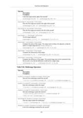


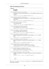
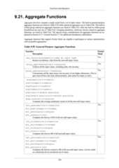

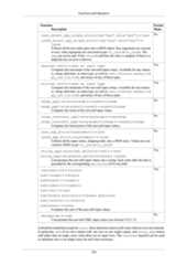


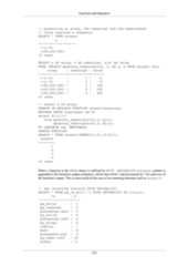
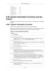


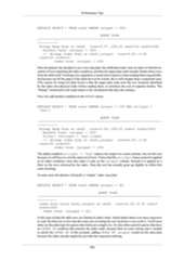


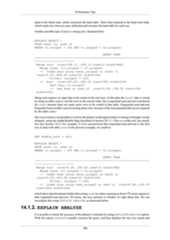


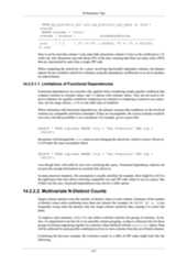
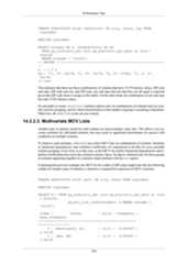


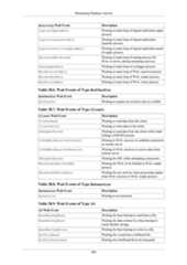


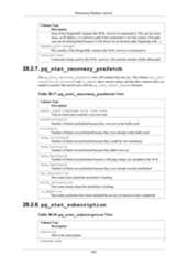
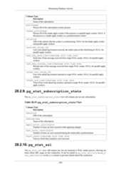

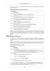
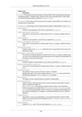


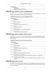


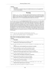
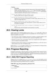


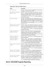


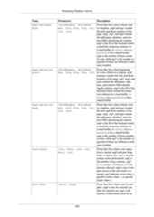


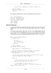
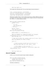


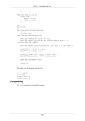


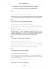


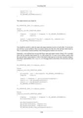
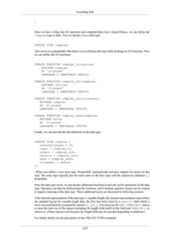


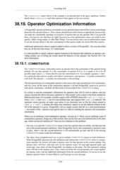


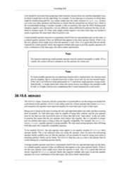


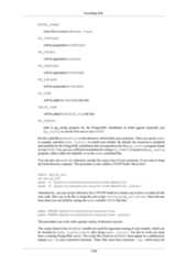
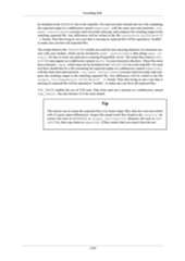


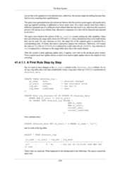


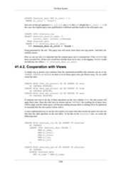
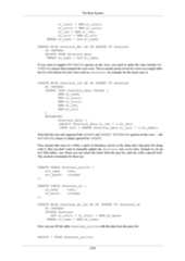


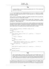


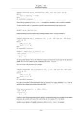


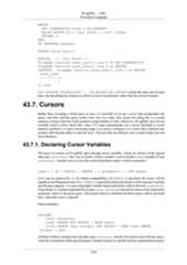


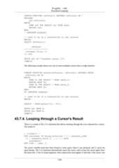
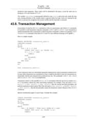


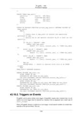


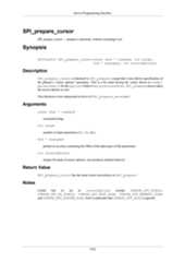
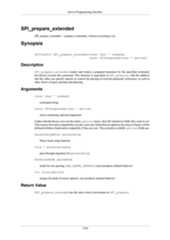

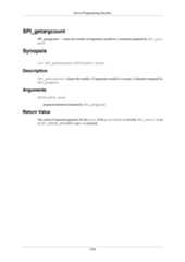


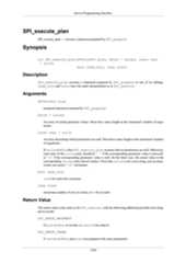


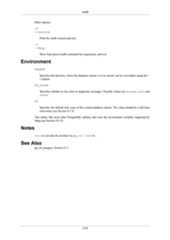


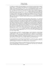
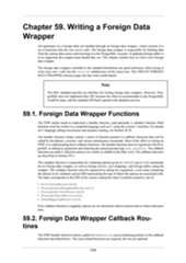
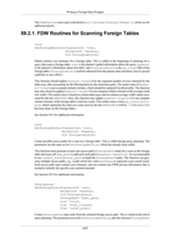
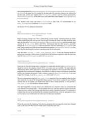


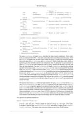


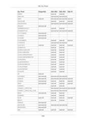


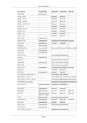
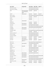


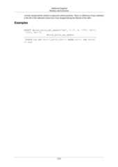


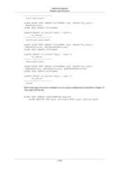


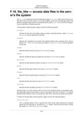


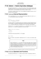
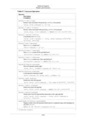


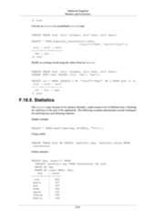


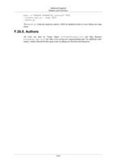


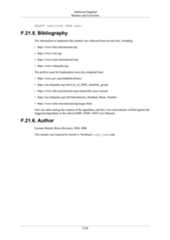


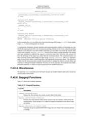


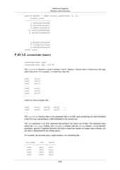


The PostgreSQL 16.3 documentation provides comprehensive information about the database system, including installation, architectural fundamentals, and SQL language fundamentals. It covers advanced features, server administration, performance tips, and data manipulation, among other topics. This documentation serves as a detailed resource for users to understand and utilize PostgreSQL effectively.


