Populations with different modes of reproduction

As a starting point, we consider the simple equation derived byWright (1938), which takes account of the variance of the contributions from parents to progeny in a population of constant sizeN,

This expression also assumes a population either containing only hermaphrodites or comprising equal numbers of males and females, diploid autosomal inheritance and random mating (including selfing for hermaphrodites). InEquation (1), the term accounts for the genetic drift caused by the variable contributions among parents, whereas the first term ‘2' in the denominator accounts for the genetic drift caused by the Mendelian segregation of heterozygotes (that is, the drift in allele frequency arising from the fact that the progeny from a heterozygote can alternatively receive one or the other allele). It can also be seen as the variance in contributions between paternal and maternal genes at a locus within an individual or part of the variance in contribution between grandparents (the termδ² inEquation (2) ofWang and Hill (2000)).

An illustrative generalisation ofEquation (1) to the case of different numbers of males (N_m) and females (N_f) is

with

where is the variance of the number of offspring of sexy from parents of sexx andS_xm,xf is the covariance of the numbers of male and female offspring from parents of sexx.Equation (2) is the same as that derived byHill (1979), although it is expressed in a different form. It reduces to the classical equation ofWright (1933,1939) for a Poisson distribution of progeny number (that is, for sexx,y=m,f),

which shows that unequal numbers of males and females in a population introduce a systematic variance in contribution between male and female parents and thus a reduction in effective size.

Predictive formulae for the effective size of X-linked genes were originally given byWright (1933) and later extended by other authors (seeCaballero, 1995). Later developments have also been made for Y-linked and maternally transmitted genes (Charlesworth, 2001;Laporte and Charlesworth, 2002;Evans and Charlesworth, 2013).

The generalisation ofEquation (1) to the case of a partially selfed population (in which there is partial selfing with proportionβ, random mating otherwise) is

(Crow and Morton, 1955), where

(Haldane, 1924) quantifies the deviation from Hardy–Weinberg equilibrium or the correlation of genes within individuals relative to the genes taken at random from the population (Wright, 1969). The value ofα in a large random mating population is approximately 0 (slightly negative when second-order terms are considered; seeEquation (23) below andWang, 1996a). For the case of biparental inbreeding such as partial full-sib mating in dioecious species, the expression is the same asEquation (5) except that the term (1+α) should be replaced by (1+3α) (Caballero and Hill, 1992). The equilibrium value ofα for biparental inbreeding is also different fromEquation (6) (for example,Ghai, 1969).

The generalisation ofEquation (5) for different numbers of males and females was made byWang (1996b), adding some covariance terms not considered byCaballero (1994) (Equation (17)). Equation byWang (1996b) also allows for different numbers of males and females varying over generations.

An excess of inbred matings (α>0 inEquation (5)) has the effect of increasing the correlation of genes within individuals and decreasing the frequency of heterozygotes by a factor ofα. It results in a decrease in the genetic drift owing to a decrease in Mendelian segregation variance and an increase in the genetic drift owing to an increase in the variance of contributions among individuals. Compared with random mating (α=0), whether an excess (α>0) or a deficit (α<0) of inbred matings may increase or decreaseN_e depends on the variance in family size,. For the case of partial selfing (Equation (5)), inbreeding (α>0) increasesN_e when and decreasesN_e when. At exactly, selfing has no effect onN_e.

Predictions of the effective size for X-linked genes in non-random mating populations were given byWang (1996c).Nomura (2002a,2005b) also provided predictions of the effective size for a variety of mating systems in animals (see alsoBalloux and Lehmann (2003)). For example, for harem polygamy, where successful males generally mate with most or all of the females in their harem and the females generally mate with only one male, the effective size, for a Poisson distribution of progeny number, is better approximated by

rather than byEquation (4), showing the larger impact of male number for this type of mating system. Other predictions ofN_e for different mating systems and overlapping generations have been provided byNunney (1993).

Equation (5) can also be obtained following the concept of long-term contributions from ancestors to descendants developed byWray and Thompson (1990) in the context of populations under selection. As suggested byWoolliams and Thompson (1994) and shown byCaballero and Toro (2000,2002), the expressions can be approximated by

whereV_∞ is the variance of long-term contributions from ancestors to descendants. For random mating (α=0),V_∞=1 andN_e=N, as expected.

For a proportionβ of partial selfing, ifα is not too close to 1 (Caballero and Toro, 2000), which, when substituted intoEquation (8), givesEquation (5). When the numbers of selfed and nonselfed progeny are independently Poisson distributed, (seeNomura, 1999a for a more precise prediction), and bothEquations (5) and(8) reduce to

(Li, 1976, p. 562;Pollak, 1987;Caballero and Hill, 1992;Nordborg and Krone, 2002). For a population with Poisson distribution of family size and complete selfing,Equation (9) reduces toN_e=N/2.Equation (8) can also be applied to the scenario of partial full-sib mating with the appropriate approximation forV_∞ (Caballero and Toro, 2000).

Predictions of the effective size for populations with mixed sexual and asexual reproduction systems and discrete and overlapping generations have been developed byYonezawa (1997). Assuming a monoecious plant species carrying out asexual propagation with a proportionδ in a population of constant sizeN (that is, an average progeny number of one and two for asexual propagation and sexual reproduction, respectively),Equation (5) ofYonezawa (1997) can be rearranged to

where is the variance of the number of asexually produced progeny among plants. If there is no asexual reproduction (δ=0),Equation (10) reduces toEquation (5), as it should. If all reproduction is asexual (δ=1),Equation (10) reduces to

Interestingly, if the number of asexually produced progeny is Poisson distributed, the expression is the same as for a sexually reproducing partially selfed population where the numbers of selfed and nonselfed progeny are independently Poisson distributed, that is,Equation (9). If all individuals are homozygotes (α=1),N_e=N/2, the same as for a fully selfed population.

An extension ofEquation (10) to overlapping generations was also given byYonezawa (1997).Equation (10) assumes that sexual and asexual contributions are independent. Predictions relaxing this assumption and extensions to more complex models were given byYonezawaet al. (2000,2004). Analytical expressions for these models of mixed sexual and asexual species were also given byOrive (1993) andBallouxet al. (2003) using coalescence theory.

Predictions of effective size for haplo–diploid species can generally be made by the standard formula for sex-linked genes (see review byCaballero, 1994). Some situations occur, however, where reproduction of these species is more complex than assumed by the simplest models. For example, in many eusocial Hymenoptera species, males can be produced by workers rather than only by queens. Predictions ofN_e for this scenario have been developed byNomura and Takahashi (2012).

Populations under selection

In the absence of selection or when selection acts on a non-inherited trait, the effective size is simply a function of the variance of the number of offspring per parent, as inEquation (5). However, predictions ofN_e are more complicated when selection acts on an inherited trait, such as when artificial selection is carried out for a quantitative trait in animal or plant breeding, or when natural selection acts on fitness traits against deleterious mutations or in favour of advantageous ones. In these scenarios, the drift process is amplified over generations because the random associations originated in a given generation between neutral and selected genes remain in descendants for a number of generations until they are eliminated by segregation and recombination. This problem was first addressed byRobertson (1961) and later on by other authors (for example,Wray and Thompson, 1990;Woolliamset al., 1993;Santiago and Caballero, 1995) for directional selection in quantitative traits. Extensions of the model were made later for populations under natural selection, linkage, overlapping generations and animal breeding schemes, as will be reviewed below.

Selection assuming unlinked genes

When selection acts on an inherited trait, changes in gene frequency at a focal neutral locus are positively correlated over generations because the selective values randomly associated with the neutral locus are not completely removed by segregation and recombination from one generation to the next. For unlinked genes and weak selection, the random association generated by sampling in a single generation is halved in consecutive generations by segregation and recombination. Therefore, the accumulative selective association has a limiting value times the value of the original random association (Robertson, 1961), and the corresponding variance of the long-term contributions of copies of the neutral gene will increase by a factorQ². With regards to drift, the effective variance of contributions of individuals (with average 2) increases owing to selection by the same factor up to 4Q²C², where the termC² is the genetic variance of the individual trait measures (for the quantitative trait subject to artificial selection or fitness-related traits in the case of natural selection) relative to the mean of the trait in the population. This variance has to be added to the expected variance of random contributions not caused by selection to predict the total variance of contributions. In reality, the associations are also reduced each generation to a proportion equal to the fraction of genetic variance remaining after selection (G), which, in turn, can be increased by the correlation between the selective advantages of male and female parents (r), and the series becomes

(Santiago and Caballero, 1995). In the case of partial selfing (or partial full-sib mating), the termr inEquation (12) should be replaced byβ (the proportion of inbred matings), because the correlation between the expected selective values of males and females (r) is approximately 1 for inbred matings (which take place with proportionβ) and approximately 0 for non-inbred matings, that is,Q=2/(2−G(1+β)).

Therefore, the equation accounting for selection as an extension ofEquation (5) is

Nomura (1999b,2005a) showed thatEquation (13), obtained by a genetic drift approach, could also be derived from an inbreeding approach by considering the variance of long-term contributions as used byWray and Thompson (1990) andWrayet al. (1990), when appropriate corrections are made in the latter (see alsoWoolliams and Bijma, 2000).

The application to different numbers of males and females was given bySantiago and Caballero (1995). That equation, however, lacked the same covariances as the equation without selection, as shown byNomura (1997a) andWang (1998). For random mating (α=0) and Poisson distribution of family sizes,Equation (13) reduces to the simplest expression (Robertson, 1961),

Equation (14) can be expressed in terms of heritability (h²) of fertility, as shown byNei and Murata (1966) andNomura (2002b). LetV_k be the observed variance of family sizes, which would be if the decay in the cumulative effect of selection is ignored (that is,Q=2). The first term,, is the non-heritable component of this variance, and the second term, 4C²=V_kh², is the heritable component. Thus substituting these intoEquation (14) yields

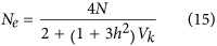(Nei and Murata, 1966). The extension ofEquation (15) to dioecious populations was developed byNei and Murata (1966) assuming random union of gametes. A more general equation was developed byNomura (2002b), who also suggested a form of the equation that avoids estimating the heritability,

wherecov_k,f andcov_k,m are the offspring–mother and offspring–father covariances of sibship size, respectively.

The prediction of effective population size under selection with overlapping generations was considered byNomura (1996) andBijmaet al. (2000). As for the non-selection case (Hill, 1979),N_e is the same as that for populations with discrete generations having the same non-selective and selective components of variance in lifetime progeny numbers and the same number of individuals entering the population each generation. Another interesting result is that the average age of parents in populations under selection is smaller than that in populations under no selection, as, in the former, younger parents tend to have higher selective advantages.

Genetic marker data can be used to assist selection (that is, marker-assisted selection (MAS)) for a quantitative trait.Nomura (2000) investigated the predictive equation ofN_e in this scenario and showed that it depends on the relative values of the genetic (r, 0.5 for full-sib families) and phenotypic (t) correlation between family members, wheret≈h²/2+c²,h² is the trait heritability andc² is the fraction of the phenotypic variance owing to the shared common environments of family members. When an index (I) is considered using individual phenotype (P) and molecular marker (M) information with given weights, that is,I=B_PP+B_MM, the effective size with MAS is reduced relative to that for phenotypic selection alone (Equation (14)) whent<r and is increased whent>r.

The prediction of effective population size under index selection was addressed byWrayet al. (1994),Caballeroet al. (1996b) andNomura (1998b,2005a). Assume truncation selection is carried out based on an index selection of the individual phenotype (P) and the mean phenotype of its full-sib family (P_f, including the individual),I=B_w(P−P_f)+B_b(P_f), whereB_w andB_b are the corresponding selection weights. The effective size can then be predicted usingEquation (14), whereQ=2/(1+kB_b) and, whereρ_I is the correlation of full sibs for the index values,ρ_A is the correlation of full sibs owing to the breeding value of the parents,k=i(i−x),i is the selection intensity andx is the truncation point in the standardised normal distribution. This predictive equation corrects a typographical error in a sign in the equation ofCaballeroet al. (1996b, p. 77). When the whole pedigree information is available, estimation of breeding values can be made by Best Linear Unbiased Prediction selection. Predictions of the effective size under this selection method were investigated byNomuraet al. (1999)Bijma and Woolliams (2000) andBijmaet al. (2001).

Other extensions for the prediction of the effective population size under selection refer to sex-linked loci (Nomura, 1997b;Wang, 1998), gynodioecious species (that is, species which have both hermaphrodite and female individuals,Laporteet al., 2000), open nucleus schemes (Nomura, 1997c;Bijma and Woolliams, 1999) and selection on traits affected by maternal effects (Rönnegård and Woolliams, 2003).

Selection at linked loci

The above formulations predict the rates of inbreeding that are usually calculated by tracing paths in genealogies of individuals. However, the real rates of inbreeding are expected to be larger than those predictions when selection acts on a system of linked genes. The reason for this is that the two gene copies at a neutral locus in an individual have different probabilities of propagation to the next generation, because they are embedded in homologous chromosomes with different alleles at linked selected loci. The problem of predictingN_e in populations under purifying selection with linkage (the background selection model;Charlesworth, 2013) was addressed byHudson and Kaplan (1995) andNordborget al. (1996) focussing on the effect of selection on nucleotide diversity, bySantiago and Caballero (1998) analysing the cumulative effect of selection over generations with a genetic drift approach (the Robertson effect) and byNicolaisen and Desai (2012,2013) using the coalescence theory. All these papers derived the same equation for the asymptoticN_e, which is a function of the haploid deleterious mutation rateU, the effects of mutations and the lengthL of the whole-genome or genome segment given in Morgans,

This equation is the exponential version ofEquation (14),, which was derived from the multiplicative fitness model assumed under background selection. HereC²=Us is the variance for fitness and the cumulative term,Q, for a rate of recombinationc between the neutral and selected loci, is (Santiago and Caballero, 1998). If the focal neutral locus is located in the middle of the genome segment and the selected loci are uniformly scattered, the average value of theQ_c² terms over the segment isQ²=1/(s(s+L/2)). Substituting this andC²=Us inEquation (14), we obtainEquation (17).

It is important to note that this equation predicts the magnitude of drift or inbreeding in the long term. For the focal neutral allele, this magnitude is effectively reached after a number of generations counted since it first appeared by mutation. Until that moment, drift at the neutral locus is expected to increase with time. The increasing drift acting on neutral mutations in consecutive generations can be predicted by the partialN_e(t) values for generationt forward in time that can be calculated using the partial cumulative terms (Santiago and Caballero, 1998). An equivalent conclusion was reached byNicolaisen and Desai (2012,2013) from the point of view of the coalescent process. The consecutiveN_e(−t) values that predict the increasing probability of coalescence under selectiont generations backwards in time (thus the negative sign) reach an asymptotic value given byEquation (17) and the predictions of the partialN_e values given by both methods, forward and backward, are exactly the same for any generationt,

Illustrations of the decline inN_e(t) over generations are given in Figure 3 ofSantiago and Caballero (1998) and Figure 3 ofNicolaisen and Desai (2013). This shows that the distortion of coalescent genealogies under selection and the cumulative effect of selection over generations are both specular images of the same process. Moreover, the pattern of neutral variation in populations under selection can be predicted by accumulating the expected distributions of neutral mutations originated in all the previous generations with the corresponding consecutive effective sizes given by theN_e(t) values (Santiago and Caballero, 1998;Nicolaisen and Desai, 2012,2013). This means that the intensity of genetic drift varies over mutations that occurred at different generations backward in time. Therefore, strictly speaking, there is not a singleN_e value representing the intensity of the drift process and, consequently, the amount and spectrum of variation under selection, even in populations at mutation–selection–drift equilibrium.

If mutations are advantageous (selective sweep model), predictions are generally cumbersome, because the genetic variance at selected loci is a function of the gene frequencies. Moreover, the stochastic distribution of selective sweeps over time is far away from the constant flux of variation usually assumed to simplify derivations.Wiehe and Stephan (1993) andGillespie (2000) derived equations for the expected heterozygosity at neutral loci using a model in which recurrent favourable mutations pass quickly through the population to fixation, wiping out linked variation. The first key simplification in these derivations is that the time of fixation of favourable mutations is so short relative to the timescale of genetic drift that it can be considered as occurring instantaneously. The second simplification is that the rate of recovery of neutral variation after a selective sweep is very slow when compared with the rate of occurrence of the sweeps. The recurrent substitutions lead to a roughly constant level of neutral variation in a stochastic process that is often referred to as ‘genetic draft'. A simple solution forN_e can be obtained by directly applying the concept of variance of long-term contributions to an evolutionary timescale:

(Gillespie, 2000), whereθ is the rate of selective sweeps andy is the final frequency of the neutral copy that was initially associated with the favourable mutation when it first appeared. The frequency of this neutral copy is expected to increase toNy copies after the sweep, and the frequency of each of the other 2N−1 copies is expected to be reduced to (1−y) copies. Therefore, the variance of the expected long-term contributions for a single selective sweep is about 2Ny². As selective sweeps occur at a rateθ, the second term of the denominator inEquation (19) is the total variance of the expected long-term contributions, that is,Q²C² inEquation (14).

Effective population size in conservation practices

The concept of effective size is key to conservation genetic practices, as it summarises the past history of the population regarding inbreeding and genetic drift and provides the prospects for the sustainability of the population if the current effective size is maintained in the future. The effective population size is directly related to the statistics widely used to monitor conservation breeding schemes, such as the number of genome equivalentsN_ge≈N_e/t (Lacy, 1995), wheret is the number of generations of management.

Minimising the loss of genetic variation is one of the main objectives of captive breeding programmes. This is achieved through minimising genetic drift and, therefore, maximisingN_e. A classical strategy to follow is the equalisation of family sizes. By choosing one couple from each pair of parents, the variance of parental contributions is null, and fromEquation (1),N_e≈2N (Wright, 1938;Crow, 1954), which is twice the effective size of an unmanaged population with a Poisson distribution of family size. This is known as minimal inbreeding and it is the recommended procedure for applications in germplasm collection and regeneration in plants (see, for example,Vencovskyet al., 2012). However, effective sizes >2N can actually be obtained by population subdivision (Wright, 1943;Wang and Caballero, 1999) and other strategies, as shown below. The extension of the strategy in the case of different numbers of males and females was developed byGoweet al. (1959). In their selection scheme, each male contributes one son andr_fm=N_f/N_m daughters, and each female contributes one daughter and has a probability ofN_m/N_f of contributing one son. Thus and all of the other variances and covariances inEquation (2) are 0. Substituting these intoEquations (2) and(3) gives

Compared with no selection (random Poisson distribution of the number of offspring per parent,Equation (4)), this scheme can increaseN_e by a proportion of (r_fm+3)/(3r_fm+1). When the female/male ratio,r_fm=N_f/N_m, is 2, for example,N_e is increased by 71.4%.

Wang (1997c) proposed an alternative design that produces further increases inN_e of about 17% whenr_fm=2. In this scheme, among ther_fm females mated with each male, one is selected at random to contribute one son and each of the remainingr_fm−1 females contributes one daughter. In this scenario, is as forEquation (20), but, and a negative covariance is induced between the numbers of male and female offspring from female parents,S_fm,ff=−N_m/N_f. Substituting these terms intoEquations (2) and(3),

The benefit of this scheme over that fromGoweet al. (1959) is decreased asr_fm gets larger. For sex-linked loci, a benefit is also produced if males are the heterogametic sex. The above equations refer to random mating of parents.Wang (1997c) also proposed a system of non-random mating in which each male is mated with one of the groups of half-sib females who are not sisters of the male. This is a sort of population subdivision where the half-sibs are like ‘subpopulations' and there is random migration of males and no migration of females among the ‘subpopulations' (seeWang and Caballero, 1999). The mating scheme can further increaseN_e over that predicted byEquation (21).

Wang (1997c) method applies to a single generation.Sánchezet al. (2003) extended the method across generations to account for long-term contributions, further improving its efficiency. With the availability of pedigree or molecular marker information, a more general method, based on finding the contributions from parents to progeny that minimise the average coancestry among the progeny (minimum coancestry contributions), is the most widely proposed criterion to maintain genetic diversity (Toro and Pérez-Enciso, 1990;Ballou and Lacy, 1995;Fernándezet al., 2003;Meuwissen, 2007). This method has been shown to minimise the variance of the long-term contributions from ancestors to descendants and, therefore, to maximise effective population size (Caballero and Toro, 2000,2002).

The above methods are all designed to reduce the variation in family sizes, the term inEquation (1) and its corresponding components when the numbers of males and females are different (Equation (2)). It is also possible to increase the effective population size by decreasing the Mendelian segregation variance, which is represented by the constant term ‘2' inEquation (1). This latter can be achieved by the use of MAS to minimise the variation in contribution between the paternally and maternally derived genes at a locus (Wang and Hill, 2000). Thus, for example, for equal numbers of males and females and equalisation of individual contributions,N_e can be expressed as

whereP_m,mf (P_f,mf) is the probability that the two genes coming from the male (female) parent and contributing to their male and female progeny are copies of the same gene. By MAS, it is possible to reduce these probabilities below the value of 0.5 expected under no control of Mendelian segregation, depending on the amount of marker information, the genome size and the number of marker-genotyped offspring per family, achieving values ofN_e>2N. MAS can also be used in a more general framework of different numbers of males and females to minimise global genetic drift and inbreeding (Wang, 2001a).

An alternative and complementary method is to use reproductive technologies for meiosis manipulation, such asin vitro culture of premeiotic germ cells and microinjection of primary spermatocytes into oocytes. By using more than one gamete from a single meiosis, variation from Mendelian segregation can be partially or completely removed (Santiago and Caballero, 2001). Thus, for example, if equalisation of family sizes is carried out and the gametes from both male and female parents are managed to come from the same meiosis in each case, the resulting effective size becomes 3N, rather than the typical 2N.

The control of the increase in inbreeding and genetic drift in conservation programmes is mainly addressed by reducing the variances of genetic contributions between paternally and maternally derived genes within and between individuals by equalising family sizes and minimising Mendelian segregation variance, as discussed above. A minor contribution to this control can also be achieved by the avoidance of inbred matings and other types of non-random mating. The simple avoidance of sib mating has a very minor effect (Wang, 1997d) and methods such as the maximum avoidance of inbreeding proposed byWright (1921) have a higher, although still relatively low, impact. These can be carried out after the design of parental contributions has been implemented (Caballeroet al., 1996a;Meuwissen, 2007). Alternatively, avoidance of inbreeding and optimal parental contributions can be realised in a single step (Fernándezet al., 2004) by the so-called mate selection method. Systems of mating involving circular (half-sib mating) (Kimura and Crow, 1963b;Theodorou and Couvet, 2010) or rotational schemes (Nomura and Yonezawa, 1996) generally reduce the ultimate rate of inbreeding but at the cost of higher initial rates (Robertson, 1964), so that their use in conservation is not recommended because of the high risk of extinction from inbreeding depression. Some methods are of particular application in selection programmes, such as the compensatory mating proposed bySantiago and Caballero (1995), where individuals from large families are mated to individuals from small ones. This produces negative correlations between the drift caused by selection and the drift caused by sampling, partly counteracting the cumulative effect of selection represented by the termQ inEquation (12). This system of mating in combination with maximum avoidance of inbreeding allows for a substantial reduction of inbreeding (Caballeroet al., 1996a).

A conservation strategy of high relevance in fisheries is supportive breeding (Hareet al., 2011), where a population is typically divided into a captive and a wild group and the offspring of the captive group are released into the wild habitat to mix with the offspring from the wild group. Because the captive group (permanent or transitional) is bred to produce a lot of offspring that are released into the wild group at each generation, the variance in family size is greatly elevated artificially and thus theN_e of the entire population is reduced. Ironically, the more successful the supportive programme is in augmenting the wild population, the greater the reduction inN_e and the greater the loss of genetic diversity in the total population (supportive+wild). This paradox is overcome only when successful supportive breeding in augmenting the wild population is carried out over a long period of time such that the excessive drift and inbreeding in the initial generations of supportive breeding is compensated for by weaker drift and inbreeding in later generations because of the increase in census size.Ryman and Laikre (1991),Rymanet al. (1995) andWang and Ryman (2001) have provided approximations for the inbreeding and variance effective sizes, respectively, which can be different in this case, with one generation of supportive breeding.Nomura (1998a) obtained an expression ofN_e from the change in coancestry, which agrees with the variance effective size, as expected. In this scenario, with various census sizes and a mixture of groups, predictions depend, however, on the generations considered (seeRymanet al., 1999).

For endangered species in the wild, estimating the effective population size and monitoring its changes over time is important in understanding the genetic health, evaluating the risk of inbreeding and inbreeding depression and thus the risk of extinction, assessing the effectiveness of the genetic managements (for example, human-aided migration/relocation, habitat protection or modification) and projecting the future demographic trajectories of the populations. Simulations (Tallmonet al., 2010) showed that monitoring the effective size is most often a more robust means of identifying stable and declining populations than monitoring census size. If a population is detected to have a small or decliningN_e, the managers of the populations should be alerted to investigate the causes and to take effective measures for reversing the course. Using noninvasive sampling (for example, from faeces, feathers, hair and so on), genetic marker data can be obtained from a population even without observing (disturbing) the animals. The data can then be analysed normally, except for accounting for the possibility of genotyping errors and allowing for a high frequency of missing data (for example,Wang, 2004), in estimatingN_e. For example, in a long-term monitoring project,Kamathet al. (2015) sampled and genotyped (at 20 microsatellite loci) 729 Yellowstone grizzly bears (Ursus arctos) born in the period 1962–2010 from an isolated and well-studied population in the Greater Yellowstone Ecosystem. They used the data to study the population demographic trajectories, estimating the changes inN_e and generation interval, over this time period.

Heterozygosity excess

Compared with an infinitely large population at Hardy–Weinberg equilibrium, a population generated from a number ofN_m male parents and a number ofN_f female parents is expected to show a deficit of homozygotes and an excess of heterozygotes at a neutral locus whenN_m,N_f or both are small. This is because male and female parents are expected to have different allele frequencies owing to drift. The smaller the value ofN_m orN_f, the greater the difference between paternal and maternal allele frequencies and thus the greater the excess in heterozygosity of the offspring population. There is a simple functional relationship between theN_e of the parental population and the amount of heterozygosity excess in the offspring population (for example,Robertson, 1965;Wang, 1996a). For a Wright–Fisher ideal population except for separate sexes withN_m male andN_f female parents, the heterozygosity excess is expected to be

whereN_e=4N_mN_f/(N_m+N_f) is the effective size of the parental population given byEquation (4). The value ofD is negative, indicating an excess of heterozygosity and a corresponding deficit of homozygosity. For a non-ideal population with arbitrary distributions of family sizes,Equation (23) is still valid whenN_m andN_f are replaced byN_em andN_ef, respectively, the effective numbers of male and female breeders.

Equation (23) suggests that measuring the heterozygosity excess,D, at a number of marker loci in a population yields an estimate of the parental population effective size.Pudovkinet al. (1996) proposed such aN_e estimator by accounting for the sampling effect,

where the observed heterozygosity excess is estimated by, is the expected heterozygosity from the observed gene frequency and is the observed heterozygosity. is calculated for each allele in a multiallelic locus and for each locus, and the average value is used inEquation (24) (Luikart and Cornuet, 1999). The accuracy of the estimator was evaluated byPudovkinet al. (1996) using simulations and was applied to a few empirical data sets (Luikart and Cornuet, 1999). The method is simple and is implemented in several computer programs (for example,Zhdanova and Pudovkin, 2008;Jones and Wang, 2010;Doet al., 2014). However, the method has a low precision and accuracy, frequently providing infinitely large estimates ofN_e for small populations. The estimator is also highly sensitive to non-random mating (for example, population subdivision, close relative mating), which also causes deviation from Hardy–Weinberg equilibrium. Its poor performance renders it useless in applications to empirical data set analysis, except when the actual population size is very small and marker information is ample.

Linkage disequilibrium

In a large unselected random mating population, alleles are independent within and between loci, producing Hardy–Weinberg equilibrium and linkage equilibrium. In a finite population, however, random genetic drift leads to associations between alleles at a locus and between alleles of different loci. The former results in heterozygosity excess, and the latter leads to gametic LD. In addition to drift, LD can also be induced by factors such as migration and direct or indirect (for example, hitchhiking) selection (Hedricket al., 1978). For neutral loci unlinked with selected loci in an isolated population under random mating, LD would come exclusively from genetic drift and can be used to estimateN_e (Hill, 1981).

An LD estimator ofN_e for a random mating population at equilibrium is based on the formulation (Hill, 1981),

wherec is the recombination rate (c=1/2 for unlinked loci),r is the correlation of allele frequencies between two loci owing to LD andn is the sample size (number of sampled individuals). In an equilibrium population, allele frequencies at two neutral loci are expected to be uncorrelated (that is,E[r]=0), such that the expectation of squaredr,E[r²], is equal to the variance ofr,V[r].Equation (25) shows thatV[r] is composed of two distinctive parts. The first comes from genetic drift, determined byN_e and linkagec. The second comes from sampling, determined by sample sizen. Using the genotypes at a number of loci ofn sampled individuals, we can estimateV[r], which can then be inserted inEquation (25) to obtain an estimate ofN_e if the recombination fractionc between loci is known. Note that a slightly different expression for the populationV[r] (that is, the first part on the right-hand side ofEquation 25) was derived bySved (1971) from an identity by descent approach. For a dioecious population with monogamy, the right side ofEquation (25) should be increased byc/(2N_ec(2−c)) (Weir and Hill, 1980).

Hill (1981) also derived the formula for the sampling variance of the estimator such that uncertainties of theN_e estimates can also be evaluated. For the case of no linkage,Waples (2006) showed by simulations that the LD estimator can seriously underestimateN_e when sample size is small. He derived empirical equations to correct for the bias caused by small sample sizes and showed by simulations that the accuracy of the modified estimator is comparable to the temporal method described in the next section. To facilitate the applications of the LD estimator,Waples and Do (2008) published a computer program, LDNE, and further evaluated its performance in comparison with the temporal method, using simulated data (Waples and Do, 2010). They concluded that, under similar conditions in terms of marker information and the actual population size, LD estimator can yieldN_e estimates that have equivalent or better qualities than the temporal estimators, except when the sampling interval of the temporal method is long.

The LD estimator is simple to calculate and requires just a single sample of multilocus genotypes instead of two or more samples, as is with the temporal method (see below). It is especially suitable for species with a long generation interval where obtaining two samples separated by a couple of generations means many years and for genetic monitoring (Schwartzet al., 2007) to track population trajectories on a yearly basis. As a result, the LD estimator has gained popularity in recent years (Palstra and Ruzzante, 2008;Luikartet al., 2010). However, some assumptions inherent to the LD estimators are often violated in real populations and as a result may lead to biasedN_e estimates. For example, it is assumed that LD is produced solely from the finite population size, and other confounding factors, such as non-random mating and population structure, are absent. Any departure from random mating (for example, an excess or deficit of close relatives mating including selfing) will affect LD and thus LD-based estimates ofN_e.Wapleset al. (2014) evaluated the effect of age structure on LD estimators and found that LD calculated from mixed-age adult samples is overestimated and thusN_e is underestimated in all of the 21 simulated species with different life tables. Similarly, the LD in a subpopulation is reduced by a constant and high rate of immigration and elevated by a low rate of immigration, compared with that of an isolated population of the sameN_e. Therefore, as observed byWaples and England (2011) in their simulation study, LD calculated from a sample from a subpopulation leads to an overestimate or an underestimate of localN_e when immigration rate is high or low, respectively. In the former case, the estimated localN_e converges to the globalN_e of the entire population (Waples and England, 2011).

LD is highly dependent on the recombination rate between loci (Hill, 1981). Pairs of closer linked loci have higher LD and thus provide better information aboutN_e (suitably defined in timescale) if the linkage information among loci is known. AlthoughHill (1981) derived his LD estimator ofN_e allowing for an arbitrary level of linkage and he advocated the use of linked markers, most often unlinked markers are used in practice because either truly unlinked markers are used or potentially linked markers are used but their linkage relationship is unknown. LD of markers of different recombination rates sheds light on the effective size of the population in different time periods in the past (Wang, 2005). Quite a few methods (Hayeset al., 2003;Barbatoet al., 2015;Mezzavilla and Ghirotto, 2015;Sauraet al., 2015) have been developed to exploit the LD information from many densely spaced markers on a chromosome segment in inferring theN_e at different time points in the past.

Temporal changes in allele frequency

For an infinitely large population under Hardy–Weinberg equilibrium, both allele frequencies and genotype frequencies remain unchanged over time. In reality, these frequencies never stay constant and change systematically owing to the forces of mutation, selection and migration, stochastically due to the random force of genetic drift, or both. In the absence of the action of all of the systematic forces in a population, any observed allele frequency change must come solely from genetic drift and can thus be used to infer the rate of drift or theN_e of the population. Based on this logic,Krimbas and Tsakas (1971) proposed to measure allele frequency changes at a number of marker loci between two temporally separated samples of individuals and thereby to estimate theN_e of the population during the sampling interval. This so-called ‘temporal method' was subsequently developed by many others in both (allele frequency) moment (for example,Nei and Tajima, 1981;Pollak, 1983;Waples, 1989) and likelihood (for example,Williamson and Slatkin, 1999;Andersonet al., 2000;Wang, 2001b;Berthieret al., 2002;Beaumont, 2003b;Lavalet al., 2003) approaches.

Moment estimators calculate a standardised variance in the temporal changes of allele frequency,F, from marker genotypes in two temporally spaced samples.F is essentially similar to Wright'sF_ST, the differences being thatF measures the temporal differentiation for the same population and it also includes sampling effect. There are a fewF estimators (for example,Nei and Tajima, 1981;Pollak, 1983) available, the one being widely applied was derived byNei and Tajima (1981). This estimator is calculated by

for a locus withk alleles, wherex_i andy_i are the observed frequencies of allelei in the first and second samples, respectively. For multiple loci, is obtained by averaging single-locus estimates. The expectation of depends on the sampling schemes (sampling with or without replacements) and is a function ofN_e and sample sizes to account for genetic drift and sampling effects. Solving the expectation equation of forN_e yields the temporal estimate of the (harmonic) meanN_e during the sampling period (Nei and Tajima, 1981;Waples, 1989).

Moment estimators rely on the summary statistic,F, which is simple to calculate. However, they do not use the full allele frequency information and are thus less accurate than the probabilistic methods. The latter, likelihood or Bayesian, are much more complicated in statistical modelling and in computation. In general, temporal methods provide good estimates ofN_e when it is not large, sampling interval is not too short (for example, one generation) and the assumptions of the methods are satisfied, using a typical set of 10–20 microsatellites. Likelihood methods generally have higher accuracy and precision than moment methods, especially for markers with rare alleles, as verified by several extensive simulations (for example,Wang, 2001b;Berthieret al., 2002;Tallmonet al., 2004). They are, however, much more computationally demanding than moment methods, which complete an analysis almost instantly. Recently, the computational efficiency of likelihood methods has been improved substantially byHui and Burt (2015), using a hidden Markov algorithm and applying continuous approximations to allele frequencies and transition probabilities. The new method can deal withN_e values as high as several millions and is implemented in an R package called NB.

A constraint on the applications of temporal approaches is the requirement of at least two samples taken at one or preferably more generations apart. The longer this sampling interval,t, is, the stronger the drift signal will be in the temporal data and the more accurate theN_e estimate will become. The extent of drift is proportional tot and is inversely proportional toN_e. For the same population and the same sampling intensity (in terms of the number of markers, number of samples and number of individuals per sample), increasing the sampling intervalt could improve the accuracy of the temporal methods tremendously, as has been repeatedly verified by simulations (for example,Nei and Tajima, 1981). Moment estimators have especially low accuracy whent is small (say,t<3) because of the weak drift signal and also because of the approximations made to the estimators. In practice, it is unfortunately difficult or unrealistic to increaset, especially for long-lived species having a long generation interval.

Compared with otherN_e estimating approaches, the temporal approach makes fewer assumptions and is more robust to some complications (realities) in real populations. For example, the approach is robust to population structure. It applies to a single unsubdivided population under non-random mating (including selfing) and to a subdivided population when sampling is representative and the aim is to estimate theN_e of the entire subdivided population rather than that of a single subpopulation. It is also robust to age structure in a population with overlapping generations, so long as the sampling intervalt is large (for example,Nei and Tajima, 1981). Whent is small, however,Waples and Yokota (2007) showed by simulations that typical sampling regimes (sampling only newborns, only adults and all age classes in proportions) result in biasedN_e estimates.Jorde and Ryman (1995) developed a moment estimator ofN_e applicable to populations with overlapping generations. They derived an age–structure correction factor, which, when applied to the standard moment estimator for populations with discrete generations, leads to unbiasedN_e estimates for populations with overlapping generations. Unfortunately, however, the correction factor is a function of numerous age-specific survival rates and age-specific reproduction rates of the focal population. These rates are usually unknown. In fact, once all these rates are known for a population, theN_e of the population can be calculated from standardN_e prediction equations (for example,Felsenstein, 1971;Hill, 1972,1979) without the need of genetic data. A method to calculate theN_e of a population with overlapping generations from its demographic parameters has been implemented in an R-package Neff (Grimmet al., 2016).

The standard temporal approach for a single unsubdivided population was also extended to estimate theN_e of a subpopulation that is connected to other subpopulations by gene flow (Wang and Whitlock, 2003). Although both drift and immigration change allele frequencies of a subpopulation, the detailed patterns of the changes are different between drift and immigration. Using temporal samples from a focal subpopulation and a sample from a large source population (the island–mainland model) or from two focal subpopulations (the island–island model), a moment estimator and a likelihood estimator can yield joint estimates ofN_e and migration rates,m. Simulations showed (Wang and Whitlock, 2003) that both moment and likelihood estimators gave reasonably good estimates ofN_e andm under typical sampling intensities. However, no estimators are available for the more general case of multiple (n>2) subpopulations. Part of the difficulty is with the number,n², of parameters to be jointly estimated, includingn effective sizes andn(n−1) migration rates. More work is badly needed in this direction as spatial and temporal genotype data are becoming easy to collect thanks to the rapid developments in molecular technologies.

One of the assumptions in the temporal approach is the absence of selection so that any change in allele frequency comes solely from drift and thus indicates the effective size of the population. For most marker loci, the assumption is valid, especially for a small population over a short sampling interval of just a few generations. However, over a long period, some loci could be affected by adaptive selection or purging selection and their allele frequencies could change faster or slower than those of neutral loci unaffected by selection. Allele frequencies at neutral loci could also evolve faster or slower because of LD with those under selection. The temporal methods have been extended to estimateN_e of a population and the selection coefficient,s, of a locus from time series data of allele frequencies (for example,Bollbacket al., 2008;Mathieson and McVean, 2013;Follet al., 2015). These methods are usually Bayesian, based on hidden Markov models to explain the observed allele frequency changes owing to drift and selection. How well these methods perform has yet to be checked, perhaps by a simulation study.

Relatedness and relationship

The pattern of genetic relatedness or relationship between individuals in a population has a direct functional relationship with the inbreeding effective size of the population (Wang, 2009). Two individuals taken at random from a population with a smallerN_e will have a higher probability of sharing the same father, mother or both. More generally, the mean and variance in pairwise relatedness within a generation are expected to increase with decreasingN_e. Based on this logic,Nomura (2008) proposed a method to use the increase in average coancestry between two consecutive generations to estimateN_e. He showed by simulations that his coancestry method is more biased but more precise than the heterozygosity excess method. The overall accuracy (measured by mean squared errors) of the two methods is similar. A major problem which causes the bias of the method, as recognised byNomura (2008), is that some non-sib pairs must be selected from a sample of individuals to act as reference in estimating the mean coancestry. The selection of non-sib pairs is difficult and somewhat subjective, because it is now well known that classifying dyads into even well-separated relationship categories, for example, full sibs, half sibs, parent offspring and unrelated, from pairwise relatedness estimates is highly error prone (for example,Blouinet al., 1996). Although many marker-based pairwise relatedness estimators are unbiased, they have high sampling errors with no exceptions (Wang, 2014).

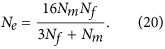
A more robust and powerful method is to estimate the frequencies of half-sib (sharing a single parent) and full-sib (sharing both parents) dyads,Q_HS andQ_FS, in a sample taken at random from a single cohort of a population (Wang, 2009;Waples and Waples, 2011).Wang (2009) derived a formula ofN_e in terms of half- and full-sib frequencies using both an inbreeding and a drift approach,

The equation has the parameterα as inEquation (5), so that theN_e for a population under non-random mating (for example, partial selfing) can be estimated. WhileQ_HS andQ_FS can be estimated from a sibship assignment analysis of the multilocus genotypes (Wang and Santure, 2009;Jones and Wang, 2010),α can be estimated from the same data with anF_ST-like approach (Wang, 2009). Alternatively,α can be assumed to be 0 for an outbred population when marker genotype frequencies do not deviate significantly from those expected under Hardy–Weinberg equilibrium. The difficulty comes from the estimation of the numbers of breeding males,N_m, and females,N_f, because sibship analysis generally makes no distinctions between paternal and maternal sibships from autosomal marker data, except in some specific situations (Wang, 2009). However, as detailed inWang (2009), the bias brought about by the last term ofEquation (27),, is usually negligible becauseα is usually small and the estimate of by a sibship analysis is also not too far from its true value.

There are several advantages of this sibship approach compared with other single-sample approaches toN_e estimation. First, sibship can be inferred more accurately than other quantities such as relatedness, which leads to more accurate estimates ofN_e. Second, the approach applies to non-random mating populations, as an inbreeding coefficientα (Equation (5); equivalent to Wright'sF_IS) can be calculated from the genotype data and incorporated into theN_e estimate. Similarly, the approach is also robust to population subdivision, as discussed byWang (2009). Third, it applies to diploid species, haplodiploid species, dioecious as well as monoecious species with selfing. Fourth, a great advantage is that it provides not only an estimate of the summary parameterN_e but also some information about the numbers of male and female parents and variance in family sizes through the sibship assignment analysis. This detailed information is especially valuable for conservation management, as a lowN_e owing to high variance in family size or a low number of parents would imply different management strategies. Simulations verified that the approach is much more accurate than the heterozygosity excess method and is similar in accuracy to the temporal methods (Wang, 2009). However, it is unclear how its accuracy compares with that of the LD method. More work is needed to clarify this issue.

The above sibship frequency approach assumes a population with discrete generations. For a population with overlapping generations, the estimate provided by the sibship frequencies in a sample of single-cohort individuals is the effective number of breeders,N_b. This parameter summarises the effects of variation in reproductive success between age classes, between sexes and between individuals within an age–sex class on genetic drift in a single breeding season, instead of in a lifetime. It is less useful thanN_e, and no population genetic equations are in terms ofN_b. However, in the absence of an estimate ofN_e,N_b provides some information about the risks of inbreeding and loss of genetic variation in conservation populations (for example,Waples and Antao, 2014;Whiteleyet al., 2015). For the case of overlapping generations,Wanget al. (2010) proposed a parentage assignment method to estimate theN_e and generation interval from the sex, age and multilocus genotype information of a single sample of individuals taken at random from a population. Essentially, the method estimates the life table by parentage assignments, and bothN_e and generation interval are then calculated from the life table. Simulations showed that the method yields unbiased and reasonably accurate estimates ofN_e under realistic sampling and genotyping effort. Application of the method to empirical data yields sensibleN_e estimates that are supported by other sources of information from the population (Kamathet al., 2015).

Multiple sources of drift/inbreeding information

The above approaches toN_e estimation use a single source of information, such as heterozygote excess, LD, temporal allele frequency changes and sibship/parentage frequencies. Each piece of information reflects a facet of the stochastic process (genetic drift or inbreeding) and combining multiple pieces of information may potentially allow for a better delineation of the process and thus yield a more accurate estimate ofN_e.Tallmonet al. (2008) proposed to use approximate Bayesian computation (ABC) to estimateN_e from a sample of microsatellite genotypes. Their method, implemented in a computer program ONESAMP, calculates and uses eight summary statistics that are known to have functional relationships withN_e from population genetic theory or simulations. These statistics include, among others, the number of alleles per locus, expected heterozygosity, LD, Wright'sF_IS and the mean and variance of multilocus homozygosity. In essence, the ABC approach simulates populations of differentN_e and tries to find theN_e value that yields the same or similar summary statistics to those calculated from the real data.Tallmonet al. (2008) demonstrated this ABC approach by analysing an introduced increasing population of ibexCapra ibex.

It is arguable that the ABC approach uses more information than other approaches. On the one hand, it uses multiple sources of information such as heterozygosity, number of alleles and LD. However, on the other hand, for each source of information, it uses a summary statistic rather than the full information that is used by the probability methods (likelihood or Bayesian). Furthermore, it is unclear how these different summary statistics should be optimally weighted, given that these statistics are, apparently, highly correlated and may reflect the inbreeding and drift processes of different timescales. For a population changing in size, these different summary statistics are relevant forN_e in different timescales. For example,F_IS (similar to heterozygosity excess) is pertinent to the parentalN_e, and LD implicatesN_e in the past few or more generations (depending on the linkage of the markers), while the number of alleles can be determined by the ancientN_e many generations (in the order ofN_e or 1/u, whichever is smaller, whereu is mutation rate) ago. So far, an extensive simulation study to compare the accuracy of ABC and other approaches is lacking but is urgently needed.

1. Allendorf FW, Luikart GH, Aitken SN. (2013) Conservation and the Genetics of Populations. John Wiley and Sons: Chichester, West Sussex, UK. [Google Scholar]
2. Anderson EC, Williamson EG, Thompson EA. (2000). Monte Carlo evaluation of the likelihood for Ne from temporally spaced samples. Genetics156: 2109–2118. [DOI] [PMC free article] [PubMed] [Google Scholar]
3. Barbato M, Orozco-terWengel P, Tapio M, Bruford MW. (2015). SNeP: a tool to estimate trends in recent effective population size trajectories using genome-wide SNP data. Front Genet6: 109. [DOI] [PMC free article] [PubMed] [Google Scholar]
4. Ballou JD, Lacy RC. (1995). Identifying genetically important individuals for management of genetic diversity in pedigreed populations. In: Ballou JD, Gilpin M, Foose TJ (eds). Population Management for Survival and Recovery. Columbia University Press: New York, USA. [Google Scholar]
5. Balloux F, Lehmann L. (2003). Random mating with a finite number of matings. Genetics165: 2313–2315. [DOI] [PMC free article] [PubMed] [Google Scholar]
6. Balloux F, Lehmann L, De Meeus T. (2003). The population genetics of clonal and partially clonal diploids. Genetics164: 1635–1644. [DOI] [PMC free article] [PubMed] [Google Scholar]
7. Beaumont MA (2003a). Conservation genetics. In: Balding DJ, Bishop M, Cannings C (eds). Handbook of Statistical Genetics, 2nd edn. Wiley: London, UK, pp 751–766.
8. Beaumont MA. (2003. b). Estimation of population growth or decline in genetically monitored populations. Genetics164: 1139–1160. [DOI] [PMC free article] [PubMed] [Google Scholar]
9. Berthier P, Beaumont MA, Cornuet JM, Luikart G. (2002). Likelihood-based estimation of the effective population size using temporal changes in allele frequencies: a genealogical approach. Genetics160: 741–751. [DOI] [PMC free article] [PubMed] [Google Scholar]
10. Bijma P, Van Arendonk JA, Woolliams JA. (2000). A general procedure for predicting rates of inbreeding in populations undergoing mass selection. Genetics154: 1865–1877. [DOI] [PMC free article] [PubMed] [Google Scholar]
11. Bijma P, Woolliams JA. (1999). Prediction of genetic contributions and generation intervals in populations with overlapping generations under selection. Genetics151: 1197–1210. [DOI] [PMC free article] [PubMed] [Google Scholar]
12. Bijma P, Woolliams JA. (2000). Prediction of rates of inbreeding in populations selected on best linear unbiased prediction of breeding value. Genetics156: 361–373. [DOI] [PMC free article] [PubMed] [Google Scholar]
13. Bijma P, Van Arendonk JAM, Woolliams JA. (2001). Predicting rates of inbreeding for livestock improvement schemes. J Anim Sci79: 840–853. [DOI] [PubMed] [Google Scholar]
14. Blouin MS, Parsons M, Lacaille V, Lotz S. (1996). Use of microsatellite loci to classify individuals by relatedness. Mol Ecol5: 393–401. [DOI] [PubMed] [Google Scholar]
15. Bollback JP, York TL, Nielsen R. (2008). Estimation of 2Nes from temporal allele frequency data. Genetics179: 497–502. [DOI] [PMC free article] [PubMed] [Google Scholar]
16. Caballero A. (1994). Developments in the prediction of effective population size. Heredity73: 657–679. [DOI] [PubMed] [Google Scholar]
17. Caballero A. (1995). On the effective size of populations with separate sexes, with particular reference to sex-linked genes. Genetics139: 1007–1011. [DOI] [PMC free article] [PubMed] [Google Scholar]
18. Caballero A, Hill WG. (1992). Effective size of nonrandom mating populations. Genetics130: 909–916. [DOI] [PMC free article] [PubMed] [Google Scholar]
19. Caballero A, Santiago E, Toro MA. (1996. a). Systems of mating to reduce inbreeding in selected populations. Anim Sci62: 431–442. [Google Scholar]
20. Caballero A, Toro MA. (2000). Interrelations between effective population size and other pedigree tools for the management of conserved populations. Genet Res75: 331–343. [DOI] [PubMed] [Google Scholar]
21. Caballero A, Toro MA. (2002). Analysis of genetic diversity for the management of conserved subdivided populations. Conserv Genet3: 289–299. [Google Scholar]
22. Caballero A, Wei M, Hill WG. (1996. b). Survival rates of mutant genes under artificial selection using individual and family information. J Genet75: 63–80. [Google Scholar]
23. Charlesworth B. (2001). The effect of life-history and mode of inheritance on neutral genetic variability. Genet Res77: 153–166. [DOI] [PubMed] [Google Scholar]
24. Charlesworth B. (2009). Fundamental concepts in genetics: effective population size and patterns of molecular evolution and variation. Nat Rev Genet10: 195–205. [DOI] [PubMed] [Google Scholar]
25. Charlesworth B. (2013). Background selection 20 years on: The Wilhelmine E. Key 2012 invitational lecture. J Hered104: 161–171. [DOI] [PubMed] [Google Scholar]
26. Charlesworth B, Charlesworth D. (2010) Elements of Evolutionary Genetics. Roberts & Co: Greenwood Village, Colorado, USA. [Google Scholar]
27. Crow JF (1954). Breeding structure of populations. II. Effective population number. In: Kempthome O, Bancroft TA, Gowan JW, Lush JL (eds). Statistics and Mathematics in Biology. Iowa State COIL Press: Ames, Iowa, USA, pp 543–556.
28. Crow JF, Morton NF. (1955). Measurement of gene frequency drift in small populations. Evolution9: 202–214. [Google Scholar]
29. Crow JF, Denniston C. (1988). Inbreeding and variance effective population numbers. Evolution42: 482–495. [DOI] [PubMed] [Google Scholar]
30. Crow JF, Kimura M. (1970) An Introduction to Population Genetics Theory. Harper & Row: New York, USA. [Google Scholar]
31. Do C, Waples RS, Peel D, Macbeth GM, Tillett BJ, Ovenden JR. (2014). NeEstimator v2: re-implementation of software for the estimation of contemporary effective population size (Ne) from genetic data. Mol Ecol Res14: 209–214. [DOI] [PubMed] [Google Scholar]
32. Engen S, Lande R, Saether BE. (2005). Effective size of a fluctuating age-structured population. Genetics170: 941–954. [DOI] [PMC free article] [PubMed] [Google Scholar]
33. Evans BJ, Charlesworth B. (2013). The effect of nonindependent mate pairing on the effective population size. Genetics193: 545–556. [DOI] [PMC free article] [PubMed] [Google Scholar]
34. Ewens WI. (1979) Mathematical Population Genetics. Springer: Berlin, Germany. [Google Scholar]
35. Falconer D, Mackay TFC. (1996) Introduction to Quantitative Genetics. Longman: Harlow, UK. [Google Scholar]
36. Felsenstein J. (1971). Inbreeding and variance effective numbers in populations with overlapping generations. Genetics68: 581–597. [DOI] [PMC free article] [PubMed] [Google Scholar]
37. Fernández J, Toro MA, Caballero A. (2003). Fixed contributions designs versus minimization of global coancestry to control inbreeding in small populations. Genetics165: 885–894. [DOI] [PMC free article] [PubMed] [Google Scholar]
38. Fernández J, Toro MA, Caballero A. (2004). Managing individuals' contributions to maximize the allelic diversity maintained in small, conserved populations. Conserv Biol18: 1–10. [Google Scholar]
39. Fisher RA. (1965) The Theory of Inbreeding, 2nd edn. Academic Press: New York, USA. [Google Scholar]
40. Foll M, Shim H, Jensen JD. (2015). WFABC: a Wright-Fisher ABC-based approach for inferring effective population sizes and selection coefficients from time-sampled data. Mol Ecol Res15: 87–98. [DOI] [PubMed] [Google Scholar]
41. Frankham RD. (1995). Effective population size/adult population size ratios in wildlife: a review. Genet Res66: 95–107. [DOI] [PubMed] [Google Scholar]
42. Frankham R, Ballou JD, Briscoe DA. (2010) Introduction to Conservation Genetics. Cambridge University Press: Cambridge, UK. [Google Scholar]
43. Ghai GL. (1969). Structure of populations under mixed random and sib mating. Theor Appl Genet39: 179–182. [DOI] [PubMed] [Google Scholar]
44. Gilbert KJ, Whitlock MC. (2015). Evaluating methods for estimating local effective population size with and without migration. Evolution69: 2154–2166. [DOI] [PubMed] [Google Scholar]
45. Gillespie JH. (2000). Genetic drift in an infinite population: the pseudo hitchhiking model. Genetics155: 909–919. [DOI] [PMC free article] [PubMed] [Google Scholar]
46. Gossmann TI, Woolfit M, Eyre-Walker A. (2011). Quantifying the variation in the effective population size within a genome. Genetics189: 1389–1402. [DOI] [PMC free article] [PubMed] [Google Scholar]
47. Gowe RS, Robertson A, Latter BDH. (1959). Environment and poultry breeding problems. 5. The design of poultry control strains. Poul Sci38: 462–471. [Google Scholar]
48. Grimm A, Gruber B, Hoehn M, Enders K, Henle K. (2016). A model-derived short-term estimation method of effective size for small populations with overlapping generations. Methods Ecol Evol (in press).
49. Haigh J. (1978). The accumulation of deleterious genes in a population-Muller's Ratchet. Theor Popul Biol14: 251–267. [DOI] [PubMed] [Google Scholar]
50. Haldane JBS. (1924). A mathematical theory of natural and artificial selection. H. The influence of partial self-fertilisation, inbreeding, assortative mating, and selective fertilisation on the composition of Mendelian populations, and on natural selection. Proc Camb Phil Soc (Biol Sci) (later Biol Rev)1: 158–163. [Google Scholar]
51. Haldane JBS. (1939). The equilibrium between mutation and random extinction. Ann Eugen9: 400–405. [Google Scholar]
52. Hare MP, Nunney L, Schwartz MK, Ruzzante DE, Burford M, Waples RS et al. (2011). Understanding and estimating effective population size for practical application in marine species management. Conserv Biol25: 438–449. [DOI] [PubMed] [Google Scholar]
53. Hayes BJ, Visscher PM, McPartlan HC, Goddard ME. (2003). Novel multilocus measure of linkage disequilibrium to estimate past effective population size. Genome Res13: 635–643. [DOI] [PMC free article] [PubMed] [Google Scholar]
54. Hedrick P, Jain S, Holden L. (1978). Multilocus systems in evolution. Evol Biol11: 101–184. [Google Scholar]
55. Hill WG. (1972). Effective size of populations with overlapping generations. Theor Popul Biol3: 278–289. [DOI] [PubMed] [Google Scholar]
56. Hill WG. (1979). A note on effective population size with overlapping generations. Genetics92: 317–322. [DOI] [PMC free article] [PubMed] [Google Scholar]
57. Hill WG. (1981). Estimation of effective population size from data on linkage disequilibrium. Genet Res38: 209–216. [Google Scholar]
58. Hill WG, Robertson A. (1966). The effects of linkage on limits to artificial selection. Genet Res8: 269–294. [PubMed] [Google Scholar]
59. Hudson RR, Kaplan NL. (1995). Deleterious background selection with recombination. Genetics141: 1605–1617. [DOI] [PMC free article] [PubMed] [Google Scholar]
60. Hui TYJ, Burt A. (2015). Estimating effective population size from temporally spaced samples with a novel, efficient maximum-likelihood algorithm. Genetics200: 285–293. [DOI] [PMC free article] [PubMed] [Google Scholar]
61. Jones OR, Wang J. (2010). COLONY: a program for parentage and sibship inference from multilocus genotype data. Mol Ecol Res10: 551–555. [DOI] [PubMed] [Google Scholar]
62. Jorde PE, Ryman N. (1995). Temporal allele frequency change and estimation of effective size in populations with overlapping generations. Genetics139: 1077–1090. [DOI] [PMC free article] [PubMed] [Google Scholar]
63. Kamath PL, Haroldson MA, Luikart G, Paetkau D, Whitman C, Manen FT. (2015). Multiple estimates of effective population size for monitoring a long-lived vertebrate: an application to Yellowstone grizzly bears. Mol Ecol24: 5507–5521. [DOI] [PubMed] [Google Scholar]
64. Kimura M, Crow JF. (1963. a). The measurement of effective population number. Evolution17: 279–288. [Google Scholar]
65. Kimura M, Crow JF. (1963. b). On the maximum avoidance of inbreeding. Genet Res4: 399–415. [Google Scholar]
66. Krimbas CB, Tsakas S. (1971). The genetics ofDacus oleae V. Changes of esterase polymorphism in a natural population following insecticide control: selection or drift? Evolution25: 454–460. [DOI] [PubMed] [Google Scholar]
67. Lacy R. (1995). Clarification of genetic terms and their use in the management of captive populations. Zoo Biol14: 565–578. [Google Scholar]
68. Laporte V, Charlesworth B. (2002). Effective population size and population subdivision in demographically structured populations. Genetics162: 501–519. [DOI] [PMC free article] [PubMed] [Google Scholar]
69. Laporte V, Cuguen J, Couvet D. (2000). Effective population sizes for cytoplasmic and nuclear genes in a gynodioecious species: the role of the sex determination system. Genetics154: 447–458. [DOI] [PMC free article] [PubMed] [Google Scholar]
70. Laval G, SanCristobal M, Chevalet C. (2003). Maximum-likehhood and Markov chain Monte Carlo approaches to estimate inbreeding and effective size from allele frequency changes. Genetics164: 1189–1204. [DOI] [PMC free article] [PubMed] [Google Scholar]
71. Li CC. (1976) First Course in Population Genetics. Boxwood: Pacific Grove, CA, USA. [Google Scholar]
72. Luikart G, Cornuet JM. (1999). Estimating the effective number of breeders from heterozygote excess in progeny. Genetics151: 1211–1216. [DOI] [PMC free article] [PubMed] [Google Scholar]
73. Luikart G, Ryman N, Tallmon DA, Schwartz MK, Allendorf FW. (2010). Estimation of census and effective population sizes: the increasing usefulness of DNA-based approaches. Conserv Genet11: 355–373. [Google Scholar]
74. Mathieson I, McVean G. (2013). Estimating selection coefficients in spatially structured populations from time series data of allele frequencies. Genetics193: 973–984. [DOI] [PMC free article] [PubMed] [Google Scholar]
75. Mezzavilla M, Ghirotto S. (2015). Neon: An R package to estimate human effective population size and divergence time from patterns of linkage disequilibrium between SNPs. J Comput Sci Syst Biol8: O37–O44. [Google Scholar]
76. Meuwissen THE. (2007) Operation of conservation schemes. In: Oldenbroek K (ed). Utilisation and Conservation of Farm Animal Genetic Resources. Wageningen Academic. Publishers: Wageningen, The Netherlands, pp 167–193. [Google Scholar]
77. Nagylaki T. (1992) Theoretical Population Genetics. Springer: Berlin, Germany. [Google Scholar]
78. Nei M, Murata M. (1966). Effective population size when fertility is inherited. Genet Res8: 257–260. [DOI] [PubMed] [Google Scholar]
79. Nei M, Tajima F. (1981). Genetic drift and estimation of effective population size. Genetics98: 625–640. [DOI] [PMC free article] [PubMed] [Google Scholar]
80. Nicolaisen LE, Desai MM. (2012). Distortions in genealogies due to purifying selection. Mol Biol Evol29: 3589–3600. [DOI] [PubMed] [Google Scholar]
81. Nicolaisen LE, Desai MM. (2013). Distortions in genealogies due to purifying selection and recombination. Genetics195: 221–230. [DOI] [PMC free article] [PubMed] [Google Scholar]
82. Nomura T. (1996). Effective size of selected populations with overlapping generations. J Anim Breed Genet113: 1–16. [Google Scholar]
83. Nomura T. (1997. a). On the effective size of nonrandom mating populations under selection. Jpn J Biometrics18: 1–11. [Google Scholar]
84. Nomura T. (1997. b). Effective population size for a sex-linked locus in populations under selection. Math Biosci142: 79–89. [DOI] [PubMed] [Google Scholar]
85. Nomura T. (1997. c). Prediction of effective population size in open nucleus breeding systems. J Anim Breed Genet114: 333–347. [DOI] [PubMed] [Google Scholar]
86. Nomura T. (1998. a). Effective population size in supportive breeding. Conserv Biol13: 670–672. [Google Scholar]
87. Nomura T (1998b). Effective population size and inbreeding under selection. Proceedings of the MAFF International Workshop on Genetic Resources Animal Genetic Resources II; 4–5 November 1998; Tsukuba, Ibaraki, Japan. National Institute of Agrobiological Resources: Tsukuba, Japan, pp 5–24.
88. Nomura T. (1999. a). Inbreeding coefficient and effective size of finite populations with a specified proportion of sib-mating. Jpn J Biometrics83: 485–489. [Google Scholar]
89. Nomura T. (1999. b). On the methods for predicting the effective size of populations under selection. Heredity83: 485–489. [DOI] [PubMed] [Google Scholar]
90. Nomura T. (2000). Effective population size under marker assisted selection. Jap J Biometrics21: 1–12. [Google Scholar]
91. Nomura T. (2002. a). Effective size of populations with unequal sex ratio and variation in mating success. J Anim Breed Genet118: 297–310. [Google Scholar]
92. Nomura T. (2002. b). Effective size of populations with heritable variation in fitness. Heredity89: 413–416. [DOI] [PubMed] [Google Scholar]
93. Nomura T. (2005. a). Developments in prediction theories of the effective size of populations under selection. Anim Sci J76: 87–96. [Google Scholar]
94. Nomura T. (2005. b). Effective population size under random mating with a finite number of matings. Genetics171: 1441–1442. [DOI] [PMC free article] [PubMed] [Google Scholar]
95. Nomura T. (2008). Estimation of effective number of breeders from molecular coancestry of single cohort sample. Evol Appl1: 462–474. [DOI] [PMC free article] [PubMed] [Google Scholar]
96. Nomura T, Mukai F, Yamamoto A. (1999). Prediction of response and inbreeding under selection based on best linear unbiased prediction in closed broiler lines. Anim Sci J70: 273–281. [Google Scholar]
97. Nomura T, Takahashi J. (2012). Effective population size in eusocial Hymenoptera with worker-produced males. Heredity109: 261–268. [DOI] [PMC free article] [PubMed] [Google Scholar]
98. Nomura T, Yonezawa K. (1996). A comparison of four systems of group mating for avoiding inbreeding. Genet Sel Evol28: 141–159. [Google Scholar]
99. Nordborg M, Krone SM (2002). Separation of time scales and convergence to the coalescent in structured populations. In: Slatkin M, Veuille M (eds). Modern Developments in Theoretical Population Genetics: The Legacy of Gustave Malécot. Oxford University Press, Oxford, UK, pp 194–232.
100. Nordborg M, Charlesworth B, Charlesworth D. (1996). The effect of recombination on background selection. Genet Res67: 159–174. [DOI] [PubMed] [Google Scholar]
101. Nunney L. (1993). The influence of mating system and overlapping generations on effective population size. Evolution47: 1329–1341. [DOI] [PubMed] [Google Scholar]
102. Orive M. (1993). Effective population size in organisms with complex life-histories. Theor Pop Biol44: 316–340. [DOI] [PubMed] [Google Scholar]
103. Palstra FP, Ruzzante DE. (2008). Genetic estimates of contemporary effective population size: what can they tell us about the importance of genetic stochasticity for wild population persistence? Mol Ecol17: 3428–3447. [DOI] [PubMed] [Google Scholar]
104. Palstra FP, Fraser DJ. (2012). Effective/census population size ratio estimation: a compendium and appraisal. Ecol Evol2: 2357–2365. [DOI] [PMC free article] [PubMed] [Google Scholar]
105. Pudovkin AI, Zaykin DV, Hedgecock D. (1996). On the potential for estimating the effective number of breeders from heterozygote-excess in progeny. Genetics144: 383–387. [DOI] [PMC free article] [PubMed] [Google Scholar]
106. Pollak E. (1983). A new method for estimating the effective population size from allele frequency changes. Genetics104: 531–548. [DOI] [PMC free article] [PubMed] [Google Scholar]
107. Pollak E. (1987). On the theory of partially inbreeding finite populations. I. Partial selling. Genetics117: 353–360. [DOI] [PMC free article] [PubMed] [Google Scholar]
108. Pollak E. (2002). Eigenvalue effective population numbers for populations that vary cyclically in size. Math Biosci177-178: 11–24. [DOI] [PubMed] [Google Scholar]
109. Robertson A. (1961). Inbreeding in artificial selection programmes. Genet Res2: 189–194. [DOI] [PubMed] [Google Scholar]
110. Robertson A. (1964). The effect of nonrandom mating within inbred lines on the rate of inbreeding. Genet Res5: 164–167. [Google Scholar]
111. Robertson A. (1965). The interpretation of genotypic ratios in domestic animal populations. Anim Prod7: 319–324. [Google Scholar]
112. Rönnegård L, Woolliams JA. (2003). Predicted rates of inbreeding with additive maternal effects. Genet Res82: 67–77. [DOI] [PubMed] [Google Scholar]
113. Ryman N, Laikre L. (1991). Effects of supportive breeding on the genetically effective population size. Conserv Biol5: 325–329. [Google Scholar]
114. Ryman N, Jorde PE, Laikre L. (1995). Supportive breeding and variance effective population size. Conserv Biol9: 1619–1628. [Google Scholar]
115. Ryman N, Jorde PE, Laikre L. (1999). Supportive breeding and inbreeding effective number: Reply to Nomura. Conserv Biol13: 673–676. [Google Scholar]
116. Sánchez L, Bijma P, Woolliams JA. (2003). Minimizing inbreeding by managing genetic contributions across generations. Genetics164: 1589–1595. [DOI] [PMC free article] [PubMed] [Google Scholar]
117. Santiago E, Caballero A. (1995). Effective size of populations under selection. Genetics139: 1013–1030. [DOI] [PMC free article] [PubMed] [Google Scholar]
118. Santiago E, Caballero A. (1998). Effective size and polymorphism of linked neutral loci in populations under directional selection. Genetics149: 2105–2117. [DOI] [PMC free article] [PubMed] [Google Scholar]
119. Santiago E, Caballero A. (2001). Application of reproductive technologies to the conservation of genetic resources. Conserv Biol14: 1831–1836. [DOI] [PubMed] [Google Scholar]
120. Saura M, Tenesa A, Woolliams JA, Fernández A, Villanueva B. (2015). Evaluation of the linkage-disequilibrium method for the estimation of effective population size when generations overlap: an empirical case. BMC Genomics16: 922. [DOI] [PMC free article] [PubMed] [Google Scholar]
121. Schwartz MK, Tallmon DA, Luikart G. (1999). Using genetics to estimate the size of wild populations: many methods, much potential, uncertain utility. Anim Conserv2: 321–323. [Google Scholar]
122. Schwartz MK, Luikart G, Waples RS. (2007). Genetic monitoring as a promising tool for conservation and management. TREE22: 25–33. [DOI] [PubMed] [Google Scholar]
123. Sved JA. (1971). Linkage disequilibrium and homozygosity of chromosome segments in finite populations. Theor Pop Biol2: 125–141. [DOI] [PubMed] [Google Scholar]
124. Tallmon DA, Luikart G, Beaumont MA. (2004). Comparative evaluation of a new effective population size estimator based on approximate Bayesian computation. Genetics167: 977–988. [DOI] [PMC free article] [PubMed] [Google Scholar]
125. Tallmon DA, Koyuk A, Luikart G, Beaumont MA. (2008). COMPUTER PROGRAMS: onesamp: a program to estimate effective population size using approximate Bayesian computation. Mol Ecol Res8: 299–301. [DOI] [PubMed] [Google Scholar]
126. Tallmon DA, Gregovich D, Waples RS, Baker CS, Jackson J, Taylor B et al. (2010). When are genetic methods useful for estimating contemporary abundance and detecting population trends? Mol Ecol Res10: 684–692. [DOI] [PubMed] [Google Scholar]
127. Theodorou K, Couvet D. (2010). Genetic management of captive populations: the advantages of circular mating. Conserv Genet11: 2289–2297. [Google Scholar]
128. Toro MA, Pérez-Enciso M. (1990). Optimization of selection response under restricted inbreeding. Genet Sel Evol22: 93–107. [Google Scholar]
129. Vencovsky R, Chaves LJ, Crossa J. (2012). Variance population size for dioecious species. Crop Sci52: 79–90. [Google Scholar]
130. Vucetich JA, Waite TA, Nunney L. (1997). Fluctuating population size and the ratio of effective size to census population size. Evolution51: 2017–3021. [DOI] [PubMed] [Google Scholar]
131. Wakeley J. (2008) Coalescent Theory. An Introduction. Ben Roberts: Greenwood Village, Colorado, USA. [Google Scholar]
132. Wakeley J, Sargsyan O. (2009). Extensions of the coalescent effective population size. Genetics181: 341–345. [DOI] [PMC free article] [PubMed] [Google Scholar]
133. Wang J. (1996. a). Deviation from Hardy-Weinberg proportions in finite populations. Genet Res68: 249–257. [Google Scholar]
134. Wang J. (1996. b). Inbreeding and variance effective sizes for non-random mating populations. Evolution50: 1786–1794. [DOI] [PubMed] [Google Scholar]
135. Wang J. (1996. c). Inbreeding coefficient and effective size for an X-linked locus in nonrandom mating populations. Heredity76: 569–577. [Google Scholar]
136. Wang J. (1997. a). Effective size and F-statistics of subdivided populations. I. Monoecious species with partial selfing. Genetics146: 1453–1463. [DOI] [PMC free article] [PubMed] [Google Scholar]
137. Wang J. (1997. b). Effective size and F-statistics of subdivided populations. II. Dioecious species. Genetics146: 1465–1474. [DOI] [PMC free article] [PubMed] [Google Scholar]
138. Wang J. (1997. c). More efficient breeding systems for controlling inbreeding and effective size in animal populations. Heredity79: 591–599. [DOI] [PubMed] [Google Scholar]
139. Wang J. (1997. d). Effect of excluding sib matings on inbreeding coefficient and effective size of finite diploid populations. Biometrics53: 1354–1365. [PubMed] [Google Scholar]
140. Wang J. (1998). Effective size of populations under selection: some extensions. Proc 6th World Cong Genet Appl Livest Prod26: 13–16. [Google Scholar]
141. Wang J. (2001. a). Optimal marker-assisted selection to increase the effective size of small populations. Genetics157: 867–874. [DOI] [PMC free article] [PubMed] [Google Scholar]
142. Wang J. (2001. b). A pseudo-likelihood method for estimating effective population size from temporally spaced samples. Genet Res78: 243–257. [DOI] [PubMed] [Google Scholar]
143. Wang J. (2004). Sibship reconstruction from genetic data with typing errors. Genetics166: 1963–1979. [DOI] [PMC free article] [PubMed] [Google Scholar]
144. Wang J. (2005). Estimation of effective population sizes from data on genetic markers. Phil Trans R Soc B360: 1395–1409. [DOI] [PMC free article] [PubMed] [Google Scholar]
145. Wang J. (2009). A new method for estimating effective population sizes from a single sample of multilocus genotypes. Mol Ecol18: 2148–2164. [DOI] [PubMed] [Google Scholar]
146. Wang J. (2014). Marker-based estimates of relatedness and inbreeding coefficients: an assessment of current methods. J Evol Biol27: 518–530. [DOI] [PubMed] [Google Scholar]
147. Wang J, Caballero A. (1999). Developments in predicting the effective size of subdivided populations. Heredity82: 212–226. [Google Scholar]
148. Wang J, Hill WG. (2000). Marker assisted selection to increase effective population size by reducing Mendelian segregation variance. Genetics154: 475–489. [DOI] [PMC free article] [PubMed] [Google Scholar]
149. Wang J, Ryman N. (2001). Genetic effects of multiple generations of supportive breeding. Conserv Biol15: 1619–1631. [Google Scholar]
150. Wang J, Santure AW. (2009). Parentage and sibship inference from multilocus genotype data under polygamy. Genetics181: 1579–1594. [DOI] [PMC free article] [PubMed] [Google Scholar]
151. Wang J, Whitlock MC. (2003). Estimating effective population size and migration rates from genetic samples over space and time. Genetics163: 429–446. [DOI] [PMC free article] [PubMed] [Google Scholar]
152. Wang J, Brekke P, Huchard E, Knapp LA, Cowlishaw G. (2010). Estimation of parameters of inbreeding and genetic drift in populations with overlapping generations. Evolution64: 1704–1718. [DOI] [PubMed] [Google Scholar]
153. Wang Y, Pollak E. (2002). The effective number of population that varies cyclically in size. II. Overlapping generations. Math Biosci179: 161–181. [DOI] [PubMed] [Google Scholar]
154. Waples RS. (1989). A generalized approach for estimating effective population size from temporal changes in allele frequency. Genetics121: 379–391. [DOI] [PMC free article] [PubMed] [Google Scholar]
155. Waples RS. (2005). Genetic estimates of contemporary effective population size: to what time periods do the estimates apply? Mol Ecol14: 3335–3352. [DOI] [PubMed] [Google Scholar]
156. Waples RS. (2006). A bias correction for estimates of effective population size based on linkage disequilibrium at unlinked gene loci. Conserv Genet7: 167–184. [Google Scholar]
157. Waples RS, Do C. (2008). LdNe: a program for estimating effective population size from data on linkage disequilibrium. Mol Ecol Res8: 753–756. [DOI] [PubMed] [Google Scholar]
158. Waples RS, Do C. (2010). Linkage disequilibrium estimates of contemporary Ne using SNPs and highly polymorphic molecular markers: an evaluation of precision and bias. Evol Appl3: 244–262. [DOI] [PMC free article] [PubMed] [Google Scholar]
159. Waples RS, England PR. (2011). Estimating contemporary effective population size on the basis of linkage disequilibrium in the face of migration. Genetics189: 633–644. [DOI] [PMC free article] [PubMed] [Google Scholar]
160. Waples RS, Antao T. (2014). Intermittent breeding and constraints on litter size: consequences for effective population size per generation (N_e and per reproductive cycle (N_b. Evolution68: 1722–1734. [DOI] [PubMed] [Google Scholar]
161. Waples RS, Waples RK. (2011). Inbreeding effective population size and parentage analysis without parents. Mol Ecol Res11: 162–171. [DOI] [PubMed] [Google Scholar]
162. Waples RS, Yokota M. (2007). Temporal estimates of effective population size in species with overlapping generations. Genetics175: 219–233. [DOI] [PMC free article] [PubMed] [Google Scholar]
163. Waples RS, Antao T, Luikart G. (2014). Effects of overlapping generations on linkage disequilibrium estimates of effective population size. Genetics197: 769–780. [DOI] [PMC free article] [PubMed] [Google Scholar]
164. Weir BS, Hill WG. (1980). Effect of mating structure on variation in linkage disequilibrium. Genetics95: 477–488. [DOI] [PMC free article] [PubMed] [Google Scholar]
165. Whiteley AR, Coombs JA, Cembrola M, O'Donnell MJ, Hudy M, Nislow KH et al. (2015). Effective number of breeders provides a link between interannual variation in stream flow and individual reproductive contribution in a stream salmonid. Mol Ecol24: 3585–3602. [DOI] [PubMed] [Google Scholar]
166. Whitlock M, Barton N. (1997). The effective size of a subdivided population. Genetics146: 427–441. [DOI] [PMC free article] [PubMed] [Google Scholar]
167. Wiehe THE, Stephan W. (1993). Analysis of a genetic hitch-hiking model, and its application to DNA polymorphism data fromDrosophila melanogaster. Mol Biol Evol10: 842–854. [DOI] [PubMed] [Google Scholar]
168. Williamson EG, Slatkin M. (1999). Using maximum likelihood to estimate population size from temporal changes in allele frequencies. Genetics152: 755–761. [DOI] [PMC free article] [PubMed] [Google Scholar]
169. Woolliams JA, Bijma P. (2000). Predicting rates of inbreeding in populations undergoing selection. Genetics154: 1851–1864. [DOI] [PMC free article] [PubMed] [Google Scholar]
170. Woolliams JA, Thompson R. (1994). A theory of genetic contributions. Proc 5th World Cong Genet Appl Livest Prod19: 127–134. [Google Scholar]
171. Woolliams JA, Wray NR, Thompson R. (1993). Prediction of long-term contributions and inbreeding in populations undergoing mass selection. Genet Res62: 231–242. [Google Scholar]
172. Wray NR, Thompson R. (1990). Predictions of rates of inbreeding in selected populations. Genet Res55: 41–54. [DOI] [PubMed] [Google Scholar]
173. Wray NR, Woolliams JA, Thompson R. (1990). Methods for predicting rates of inbreeding in selected populations. Theor Appl Genet80: 503–512. [DOI] [PubMed] [Google Scholar]
174. Wray NR, Woolliams JA, Thompson R. (1994). Predicting of rates of inbreeding in populations undergoing index selection. Theor Appl Genet87: 878–892. [DOI] [PubMed] [Google Scholar]
175. Wright S. (1921). Systems of mating. Genetics6: 111–178. [DOI] [PMC free article] [PubMed] [Google Scholar]
176. Wright S. (1931). Evolution in Mendelian populations. Genetics16: 97–159. [DOI] [PMC free article] [PubMed] [Google Scholar]
177. Wright S. (1933). Inbreeding and homozygosis. Proc Natl Acad Sci USA19: 411–420. [DOI] [PMC free article] [PubMed] [Google Scholar]
178. Wright S. (1938). Size of population and breeding structure in relation to evolution. Science87: 430–431. [Google Scholar]
179. Wright S. (1939) Statistical Genetics in Relation to Evolution. Exposés de Biométrie et de Statistique Biologique. Herman & Cie: Paris, France. [Google Scholar]
180. Wright S. (1943). Isolation by distance. Genetics28: 114–138. [DOI] [PMC free article] [PubMed] [Google Scholar]
181. Wright S. (1969) Evolution and the Genetics of Populations, vol. 2, The Theory of Gene Frequencies. University of Chicago Press: Chicago, IL, USA. [Google Scholar]
182. Yonezawa K. (1997). Effective population size of plant species propagating with mixed sexual and asexual reproduction system. Genet Res70: 251–258. [Google Scholar]
183. Yonezawa K, Kinoshita E, Watano Y, Zentoh H. (2000). Formulation and estimation of the effective size of stage-structured populations inFritillaria camtschatcensis, a perennial herb with a complex life history. Genetics54: 2007–2013. [DOI] [PubMed] [Google Scholar]
184. Yonezawa K, Ishii T, Nagamine T. (2004). The effective size of mixed sexually and asexually reproducing populations. Genetics166: 1529–1539. [DOI] [PMC free article] [PubMed] [Google Scholar]
185. Zhdanova OL, Pudovkin AI. (2008). Nb_HetEx: a program to estimate the effective number of breeders. J Hered99: 694–695. [DOI] [PubMed] [Google Scholar]