Weight Adjustments in Practice
Michael Dumelleand Anthony R. Olsen
Source:vignettes/articles/weighting.Rmdweighting.RmdIf you have yet not read the “Start Here” vignette, please do so byrunning
vignette("start-here","spsurvey")Introduction
An important part of a statistical survey design is constructingdesign weights that are representative of the target population (i.e.,population of interest). Appropriate design weights are combined withdata collected in the field to estimate population parameters like meansand totals. At the start of a survey design, weights at a site typicallyequal the reciprocal of the site’s inclusion probability (i.e., theprobability the site was selected from the sampling frame as part of therandom sample). Thus, these weights characterize how many “similarunits” the site represents in the target population. An importantproperty of these weights is that they generally sum to\(N\), the known population size (morerigorously, the sampling frame size). However, these initial weights areoften adjusted prior to analysis, for myriad reasons that include achange to the survey design (i.e., the sample size changed partwaythrough the survey, nonresponse, and/or to improve the performance ofstatistical estimators). Here we outline some strategies for weightadjustments using a few practical examples that reflect commonecological applications. For an introduction to survey design andweighting, see Lumley (2011) and Lohr (2021); for a more technicaltreatment, see Särndal et al. (2003).
Before proceeding, we loadspsurvey and set areproducible seed by running
TheNE_Lakes data contains a population of 195 lakes inthe Northeast United States (US):
NE_Lakes#> Simple feature collection with 195 features and 4 fields#> Geometry type: POINT#> Dimension: XY#> Bounding box: xmin: 1834001 ymin: 2225021 xmax: 2127632 ymax: 2449985#> Projected CRS: NAD83 / Conus Albers#> First 10 features:#> AREA AREA_CAT ELEV ELEV_CAT geometry#> 1 10.648825 large 264.69 high POINT (1930929 2417191)#> 2 2.504606 small 557.63 high POINT (1849399 2375085)#> 3 3.979199 small 28.79 low POINT (2017323 2393723)#> 4 1.645657 small 212.60 high POINT (1874135 2313865)#> 5 7.489052 small 239.67 high POINT (1922712 2392868)#> 6 86.533725 large 195.37 high POINT (1977163 2350744)#> 7 1.926996 small 158.96 high POINT (1852292 2257784)#> 8 6.514217 small 29.26 low POINT (1874421 2247388)#> 9 3.100221 small 204.62 high POINT (1933352 2368181)#> 10 1.868094 small 78.77 low POINT (1892582 2364213)We can visualize the layout of these lakes:

Throughout, we will select both unstratified and stratified samplesfrom theNE_Lakes data and show how weights are constructedand adjusted, step-by-step. We assume the sampling frame and targetpopulation are the same, though we eventually relax this assumption toaccommodate overcoverage, which occurs when the target population isactually a subset of the sampling frame.
Weighting in Unstratified Sampling
Suppose our goal is to use a spatially balanced random sample of 10sites fromNE_Lakes to estimate the proportion of all 195lakes in “Good” benthic macroinvertebrate condition. To accomplish thisgoal, we must sample 10 lakes and determine whether the lake is in goodcondition, assign weights to each of the 10 sampled lakes, and combinethe weights with the data to estimate this proportion for all lakes.Ideally, we would select a sample of size 10 and each of these lakescould be sampled. In practice, however, there are many scenarios wherefield crews cannot sample a site, a few of which include:
- An endangered species is detected at the site
- The site is not safely accessible at the time of sampling
- The site is on private land and the field crew lacks permission fromthe landowner to sample
If it is expected that some sites cannot be sampled, it is useful toselect an “oversample” of sites that act as replacement sites to the“base” sample. Here, we select a base sample of size 10 with anoversample of size 10 fromNE_Lakes:
samp<-grts(NE_Lakes, n_base=10, n_over=10)We may visualize the spatial distribution of sites alongside theNE_Lakes population:
plot(samp, sframe=NE_Lakes, pch=19)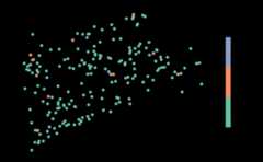
Each site has probability 10/195 of being included in the sample,which implies that each base site is assigned a weight of 195/10, or19.5
samp$sites_base[,c("siteID","siteuse","wgt")]#> Simple feature collection with 10 features and 3 fields#> Geometry type: POINT#> Dimension: XY#> Bounding box: xmin: 1844177 ymin: 2257478 xmax: 2088529 ymax: 2446688#> Projected CRS: NAD83 / Conus Albers#> siteID siteuse wgt geometry#> 1 Site-01 Base 19.5 POINT (1854595 2348778)#> 2 Site-02 Base 19.5 POINT (1914389 2407526)#> 3 Site-03 Base 19.5 POINT (2014745 2446688)#> 4 Site-04 Base 19.5 POINT (1856350 2257478)#> 5 Site-05 Base 19.5 POINT (1849399 2375085)#> 6 Site-06 Base 19.5 POINT (1981644 2350859)#> 7 Site-07 Base 19.5 POINT (2088529 2350777)#> 8 Site-08 Base 19.5 POINT (1874135 2313865)#> 9 Site-09 Base 19.5 POINT (1844177 2383131)#> 10 Site-10 Base 19.5 POINT (2048021 2385862)The sum of these weights equals 195, the known population size:
sum(samp$sites_base$wgt)#> [1] 195The base and oversample sites are combined into a singlesf object usingsp_rbind():
sites_unstrat<-sp_rbind(samp)Suppose that field crews determined that first four sites weresampleable, the fifth site was inaccessible, and so on. We store theevaluation status of each site in a variable calledEVAL_CAT, short for evaluation category:
sites_unstrat$EVAL_CAT<-c(rep("Sampleable",4),"Lack_Permission",rep("Sampleable",2),rep("Inaccessible",2),"Sampleable",rep("Lack_Permission",2),"Endangered",rep("Sampleable",2),"Lack_Permission","Sampleable",rep("Not_Needed",3))print(sites_unstrat[,c("siteID","siteuse","EVAL_CAT")], n=20)#> Simple feature collection with 20 features and 3 fields#> Geometry type: POINT#> Dimension: XY#> Bounding box: xmin: 1844177 ymin: 2239763 xmax: 2088529 ymax: 2446688#> Projected CRS: NAD83 / Conus Albers#> siteID siteuse EVAL_CAT geometry#> 1 Site-01 Base Sampleable POINT (1854595 2348778)#> 2 Site-02 Base Sampleable POINT (1914389 2407526)#> 3 Site-03 Base Sampleable POINT (2014745 2446688)#> 4 Site-04 Base Sampleable POINT (1856350 2257478)#> 5 Site-05 Base Lack_Permission POINT (1849399 2375085)#> 6 Site-06 Base Sampleable POINT (1981644 2350859)#> 7 Site-07 Base Sampleable POINT (2088529 2350777)#> 8 Site-08 Base Inaccessible POINT (1874135 2313865)#> 9 Site-09 Base Inaccessible POINT (1844177 2383131)#> 10 Site-10 Base Sampleable POINT (2048021 2385862)#> 11 Site-11 Over Lack_Permission POINT (2009223 2301696)#> 12 Site-12 Over Lack_Permission POINT (1925479 2268716)#> 13 Site-13 Over Endangered POINT (1974036 2355133)#> 14 Site-14 Over Sampleable POINT (2001212 2369527)#> 15 Site-15 Over Sampleable POINT (2005879 2336463)#> 16 Site-16 Over Lack_Permission POINT (1965198 2291328)#> 17 Site-17 Over Sampleable POINT (1961036 2381322)#> 18 Site-18 Over Not_Needed POINT (2023662 2397647)#> 19 Site-19 Over Not_Needed POINT (1865304 2239763)#> 20 Site-20 Over Not_Needed POINT (1917742 2297169)table(sites_unstrat$EVAL_CAT)#>#> Endangered Inaccessible Lack_Permission Not_Needed Sampleable#> 1 2 4 3 10In this example, 17 total sites were evaluated. In between the firstand tenth sampled site, seven sites were not sampleable (inaccessible,lacking permission, endangered species). Sites should always beevaluated insiteID order, as this is important to maximizespatial balance of the sampled sites whenn_base andn_over are both used. Because the goal of 10 sampleablesites was reached after evaluating 17 sites, the final three oversamplesites are not needed and can be removed:
sites_unstrat<-sites_unstrat[sites_unstrat$EVAL_CAT!="Not_Needed",]print(sites_unstrat[,c("siteID","siteuse","EVAL_CAT")], n=17)#> Simple feature collection with 17 features and 3 fields#> Geometry type: POINT#> Dimension: XY#> Bounding box: xmin: 1844177 ymin: 2257478 xmax: 2088529 ymax: 2446688#> Projected CRS: NAD83 / Conus Albers#> siteID siteuse EVAL_CAT geometry#> 1 Site-01 Base Sampleable POINT (1854595 2348778)#> 2 Site-02 Base Sampleable POINT (1914389 2407526)#> 3 Site-03 Base Sampleable POINT (2014745 2446688)#> 4 Site-04 Base Sampleable POINT (1856350 2257478)#> 5 Site-05 Base Lack_Permission POINT (1849399 2375085)#> 6 Site-06 Base Sampleable POINT (1981644 2350859)#> 7 Site-07 Base Sampleable POINT (2088529 2350777)#> 8 Site-08 Base Inaccessible POINT (1874135 2313865)#> 9 Site-09 Base Inaccessible POINT (1844177 2383131)#> 10 Site-10 Base Sampleable POINT (2048021 2385862)#> 11 Site-11 Over Lack_Permission POINT (2009223 2301696)#> 12 Site-12 Over Lack_Permission POINT (1925479 2268716)#> 13 Site-13 Over Endangered POINT (1974036 2355133)#> 14 Site-14 Over Sampleable POINT (2001212 2369527)#> 15 Site-15 Over Sampleable POINT (2005879 2336463)#> 16 Site-16 Over Lack_Permission POINT (1965198 2291328)#> 17 Site-17 Over Sampleable POINT (1961036 2381322)Recall our primary goal is to estimate the proportion of lakes ingood BMI condition. However, a secondary goal may be to estimate theproportion of lakes that are able to be sampled. To accomplish thisgoal, we must first adjust our original weights to reflect the fact that17 sites were evaluated. These adjusted weights must still sum to 195,the population size, and they still must be equal (as all sites had thesame probability of being included in the sample). This implies thateach weight is 195/17, or 11.47. The original weights are adjusted by ascaling factor that represents the ratio of the original sample size tothe number of evaluated sites, or 10/17. This type of weight adjustmentis available inspsurvey using theadjwgt()function:
sites_unstrat$adjwgt<-adjwgt( wgt=sites_unstrat$wgt, framesize=195)print(sites_unstrat[,c("siteID","siteuse","EVAL_CAT","adjwgt")], n=17)#> Simple feature collection with 17 features and 4 fields#> Geometry type: POINT#> Dimension: XY#> Bounding box: xmin: 1844177 ymin: 2257478 xmax: 2088529 ymax: 2446688#> Projected CRS: NAD83 / Conus Albers#> siteID siteuse EVAL_CAT adjwgt geometry#> 1 Site-01 Base Sampleable 11.47059 POINT (1854595 2348778)#> 2 Site-02 Base Sampleable 11.47059 POINT (1914389 2407526)#> 3 Site-03 Base Sampleable 11.47059 POINT (2014745 2446688)#> 4 Site-04 Base Sampleable 11.47059 POINT (1856350 2257478)#> 5 Site-05 Base Lack_Permission 11.47059 POINT (1849399 2375085)#> 6 Site-06 Base Sampleable 11.47059 POINT (1981644 2350859)#> 7 Site-07 Base Sampleable 11.47059 POINT (2088529 2350777)#> 8 Site-08 Base Inaccessible 11.47059 POINT (1874135 2313865)#> 9 Site-09 Base Inaccessible 11.47059 POINT (1844177 2383131)#> 10 Site-10 Base Sampleable 11.47059 POINT (2048021 2385862)#> 11 Site-11 Over Lack_Permission 11.47059 POINT (2009223 2301696)#> 12 Site-12 Over Lack_Permission 11.47059 POINT (1925479 2268716)#> 13 Site-13 Over Endangered 11.47059 POINT (1974036 2355133)#> 14 Site-14 Over Sampleable 11.47059 POINT (2001212 2369527)#> 15 Site-15 Over Sampleable 11.47059 POINT (2005879 2336463)#> 16 Site-16 Over Lack_Permission 11.47059 POINT (1965198 2291328)#> 17 Site-17 Over Sampleable 11.47059 POINT (1961036 2381322)The first argument,wgt, is the vector of weights, andthe second argument,framesize is\(N\), the known population size. The sum ofthese adjusted weights equals 195:
sum(sites_unstrat$adjwgt)#> [1] 195Then we could use these weights to estimate the proportion of thepopulation that is sampleable or not sampleable due to endangeredspecies, inaccessibility, or a lack of landowner permission:
out<-cat_analysis(sites_unstrat, vars="EVAL_CAT", weight="adjwgt")out[,c("Indicator","Category","nResp","Estimate.P","StdError.P")]#> Indicator Category nResp Estimate.P StdError.P#> 1 EVAL_CAT Endangered 1 5.882353 4.952669#> 2 EVAL_CAT Inaccessible 2 11.764706 6.861383#> 3 EVAL_CAT Lack_Permission 4 23.529412 7.869084#> 4 EVAL_CAT Sampleable 10 58.823529 9.744101#> 5 EVAL_CAT Total 17 100.000000 0.000000Though some sites could not be sampled, we still presume these sitesare in the target population and are either in “Good” or “Not Good” BMIcondition. To reflect this assumption, we must adjust the weights of thesampled sites to account for nonresponse (here, due to endangeredspecies, inaccessibility, or a lack of landowner permission) in thetarget population. This weight adjustment involves two parts. First, theweights are scaled by the reciprocal of the probability an evaluatedsite was sampled, or 17/10. Second, the the weights for sites that werenot sampled are set to zero. This type of nonresponse weight adjustmentis available inspsurvey using theadjwgtNR()function:
sites_unstrat$adjwgt_nr<-adjwgtNR( wgt=sites_unstrat$adjwgt, EvalStatus=sites_unstrat$EVAL_CAT, TNRClass=c("Inaccessible","Lack_Permission","Endangered"), TRClass="Sampleable")print(sites_unstrat[,c("siteID","siteuse","EVAL_CAT","adjwgt","adjwgt_nr")], n=17)#> Simple feature collection with 17 features and 5 fields#> Geometry type: POINT#> Dimension: XY#> Bounding box: xmin: 1844177 ymin: 2257478 xmax: 2088529 ymax: 2446688#> Projected CRS: NAD83 / Conus Albers#> siteID siteuse EVAL_CAT adjwgt adjwgt_nr geometry#> 1 Site-01 Base Sampleable 11.47059 19.5 POINT (1854595 2348778)#> 2 Site-02 Base Sampleable 11.47059 19.5 POINT (1914389 2407526)#> 3 Site-03 Base Sampleable 11.47059 19.5 POINT (2014745 2446688)#> 4 Site-04 Base Sampleable 11.47059 19.5 POINT (1856350 2257478)#> 5 Site-05 Base Lack_Permission 11.47059 0.0 POINT (1849399 2375085)#> 6 Site-06 Base Sampleable 11.47059 19.5 POINT (1981644 2350859)#> 7 Site-07 Base Sampleable 11.47059 19.5 POINT (2088529 2350777)#> 8 Site-08 Base Inaccessible 11.47059 0.0 POINT (1874135 2313865)#> 9 Site-09 Base Inaccessible 11.47059 0.0 POINT (1844177 2383131)#> 10 Site-10 Base Sampleable 11.47059 19.5 POINT (2048021 2385862)#> 11 Site-11 Over Lack_Permission 11.47059 0.0 POINT (2009223 2301696)#> 12 Site-12 Over Lack_Permission 11.47059 0.0 POINT (1925479 2268716)#> 13 Site-13 Over Endangered 11.47059 0.0 POINT (1974036 2355133)#> 14 Site-14 Over Sampleable 11.47059 19.5 POINT (2001212 2369527)#> 15 Site-15 Over Sampleable 11.47059 19.5 POINT (2005879 2336463)#> 16 Site-16 Over Lack_Permission 11.47059 0.0 POINT (1965198 2291328)#> 17 Site-17 Over Sampleable 11.47059 19.5 POINT (1961036 2381322)The first argument,wgt, is the vector of weights; thesecond argument,EvalStatus is the evaluation status (here,EVAL_CAT); the third argument,TNRClass, aretheEVAL_CAT values that indicate the site was not able tobe sampled; and the fourth argument,TRClass, is theEVAL_CAT value that indicates the site was sampled. The sumof these nonresponse adjusted weights equals 195, the known populationsize:
sum(sites_unstrat$adjwgt_nr)#> [1] 195Suppose that at the sampled sites, the following BMI_COND values wererecorded:
sites_unstrat_samp<-sites_unstrat[sites_unstrat$EVAL_CAT=="Sampleable",]sites_unstrat_samp$BMI_COND<-c(rep("Good",3),"Not_Good","Good",rep("Not_Good",2),rep("Good",3))print(sites_unstrat_samp[,c("siteID","siteuse","EVAL_CAT","adjwgt_nr","BMI_COND")])#> Simple feature collection with 10 features and 5 fields#> Geometry type: POINT#> Dimension: XY#> Bounding box: xmin: 1854595 ymin: 2257478 xmax: 2088529 ymax: 2446688#> Projected CRS: NAD83 / Conus Albers#> siteID siteuse EVAL_CAT adjwgt_nr BMI_COND geometry#> 1 Site-01 Base Sampleable 19.5 Good POINT (1854595 2348778)#> 2 Site-02 Base Sampleable 19.5 Good POINT (1914389 2407526)#> 3 Site-03 Base Sampleable 19.5 Good POINT (2014745 2446688)#> 4 Site-04 Base Sampleable 19.5 Not_Good POINT (1856350 2257478)#> 6 Site-06 Base Sampleable 19.5 Good POINT (1981644 2350859)#> 7 Site-07 Base Sampleable 19.5 Not_Good POINT (2088529 2350777)#> 10 Site-10 Base Sampleable 19.5 Not_Good POINT (2048021 2385862)#> 14 Site-14 Over Sampleable 19.5 Good POINT (2001212 2369527)#> 15 Site-15 Over Sampleable 19.5 Good POINT (2005879 2336463)#> 17 Site-17 Over Sampleable 19.5 Good POINT (1961036 2381322)Then we could use these nonresponse weights to estimate theproportion of lakes fromNE_Lakes in “Good” BMIcondition:
out<-cat_analysis(sites_unstrat_samp, vars="BMI_COND", weight="adjwgt_nr")out[,c("Indicator","Category","nResp","Estimate.P","StdError.P")]#> Indicator Category nResp Estimate.P StdError.P#> 1 BMI_COND Good 7 70 12.77128#> 2 BMI_COND Not_Good 3 30 12.77128#> 3 BMI_COND Total 10 100 0.00000Weighting in Stratified Sampling
Sometimes it is desired to select separate samples from distinctsubsets of the population, called strata. This type of sample is calleda stratified sample. Consider the size of lakes inNE_Lakes, represented by theAREA_CAT variablewith two levels, “small” and “large”:

There are 135 small lakes and 60 large lakes. Because there are moresmall lakes than large lakes, a random sample of size 10 may not yieldany large lakes! We could instead use a stratified sample to select fivespatially balanced sites from small lakes and five spatially balancedsites from large lakes (with five oversamples in each strata):
samp<-grts(NE_Lakes, n_base=c("small"=5,"large"=5), stratum_var="AREA_CAT", n_over=c("small"=5,"large"=5))In a stratified sample,n_base andn_overare vectors whose names represent strata and values represent samplesizes. Thestratum_var argument specifies the variable inNE_Lakes that contains the strata.
We may visualize the spatial distribution of sites alongside theNE_Lakes population (separately for each strata):
plot(samp,siteuse~AREA_CAT, sframe=NE_Lakes, pch=19)
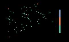
Each small (large) lake has a probability 5/135 (5/60) of beingincluded in the sample, which implies that each base site is assigned aweight of 135/5 (60/5), or 27 (12). Within each strata, the weights mustsum to\(N_{small}\) (135) and\(N_{large}\) (60), the target populationsize of small lakes and large lakes, respectively.
samp$sites_base[,c("siteID","siteuse","AREA_CAT","wgt")]#> Simple feature collection with 10 features and 4 fields#> Geometry type: POINT#> Dimension: XY#> Bounding box: xmin: 1847705 ymin: 2237642 xmax: 2030546 ymax: 2448538#> Projected CRS: NAD83 / Conus Albers#> siteID siteuse AREA_CAT wgt geometry#> 1 Site-01 Base small 27 POINT (2009223 2301696)#> 2 Site-02 Base small 27 POINT (1872450 2255923)#> 3 Site-03 Base small 27 POINT (2009953 2389537)#> 4 Site-04 Base small 27 POINT (1978886 2337620)#> 5 Site-05 Base small 27 POINT (1864944 2305864)#> 6 Site-06 Base large 12 POINT (1930547 2278764)#> 7 Site-07 Base large 12 POINT (1851496 2237642)#> 8 Site-08 Base large 12 POINT (1847705 2417128)#> 9 Site-09 Base large 12 POINT (2030546 2448538)#> 10 Site-10 Base large 12 POINT (1961036 2381322)The sum of these weights equal the appropriate population totals:
tapply( X=samp$sites_base$wgt, INDEX=samp$sites_base$AREA_CAT, FUN=sum)#> small large#> 135 60The base and oversample sites are combined into a singlesf object usingsp_rbind():
sites_strat<-sp_rbind(samp)Suppose the sites had the following evaluation status:
sites_strat$EVAL_CAT<-c(rep("Sampleable",2),"Endangered","Sampleable","Lack_Permission","Lack_Permission",rep("Sampleable",3),"Lack_Permission","Inaccessible","Sampleable","Endangered","Sampleable","Not_Needed","Lack_Permission",rep("Sampleable",2),rep("Not_Needed",2))sites_strat<-sites_strat[order(sites_strat$AREA_CAT),]In total, 9 (8) small (large) lakes were evaluated. Next, we removethe sites that were not needed:
sites_strat<-sites_strat[sites_strat$EVAL_CAT!="Not_Needed",]Each small (large) evaluated lake should have a weight of 135/9(60/8), or 15 (7.5). The original weights are adjusted to reflectevaluation category usingadjwgt():
sites_strat$adjwgt<-adjwgt( wgt=sites_strat$wgt, wgtcat=sites_strat$AREA_CAT, framesize=c("small"=135,"large"=60))print(sites_strat[,c("siteID","siteuse","AREA_CAT","EVAL_CAT","adjwgt")], n=17)#> Simple feature collection with 17 features and 5 fields#> Geometry type: POINT#> Dimension: XY#> Bounding box: xmin: 1847705 ymin: 2237642 xmax: 2093440 ymax: 2448538#> Projected CRS: NAD83 / Conus Albers#> siteID siteuse AREA_CAT EVAL_CAT adjwgt geometry#> 1 Site-01 Base small Sampleable 15.0 POINT (2009223 2301696)#> 2 Site-02 Base small Sampleable 15.0 POINT (1872450 2255923)#> 3 Site-03 Base small Endangered 15.0 POINT (2009953 2389537)#> 4 Site-04 Base small Sampleable 15.0 POINT (1978886 2337620)#> 5 Site-05 Base small Lack_Permission 15.0 POINT (1864944 2305864)#> 11 Site-11 Over small Inaccessible 15.0 POINT (1941191 2365612)#> 12 Site-12 Over small Sampleable 15.0 POINT (1929095 2335384)#> 13 Site-13 Over small Endangered 15.0 POINT (1991533 2371473)#> 14 Site-14 Over small Sampleable 15.0 POINT (2093440 2352167)#> 6 Site-06 Base large Lack_Permission 7.5 POINT (1930547 2278764)#> 7 Site-07 Base large Sampleable 7.5 POINT (1851496 2237642)#> 8 Site-08 Base large Sampleable 7.5 POINT (1847705 2417128)#> 9 Site-09 Base large Sampleable 7.5 POINT (2030546 2448538)#> 10 Site-10 Base large Lack_Permission 7.5 POINT (1961036 2381322)#> 16 Site-16 Over large Lack_Permission 7.5 POINT (1983310 2426290)#> 17 Site-17 Over large Sampleable 7.5 POINT (1886052 2287068)#> 18 Site-18 Over large Sampleable 7.5 POINT (2059943 2379491)Thewgtcat argument (which stands for weight categories)is required to adjust weights separately for each lake size category,andframesize now has names representing lake size categoryand values equaling the known target population size (within lake sizecategory).
We can check that the adjusted weights sum to the appropriatepopulation sizes:
tapply( X=sites_strat$adjwgt, INDEX=sites_strat$AREA_CAT, FUN=sum)#> small large#> 135 60We can use these weights to estimate the proportion of the populationthat is sampleable or not sampleable due to endangered species,inaccessibility, or a lack of landowner permission. We can do thisseparately for each strata:
out<-cat_analysis(sites_strat, vars="EVAL_CAT", subpop="AREA_CAT", weight="adjwgt")out[,c("Indicator","Subpopulation","Category","nResp","Estimate.P","StdError.P")]#> Indicator Subpopulation Category nResp Estimate.P StdError.P#> 1 EVAL_CAT large Endangered 0 0.00000 0.000000#> 2 EVAL_CAT large Inaccessible 0 0.00000 0.000000#> 3 EVAL_CAT large Lack_Permission 3 37.50000 16.627375#> 4 EVAL_CAT large Sampleable 5 62.50000 16.627375#> 5 EVAL_CAT large Total 8 100.00000 0.000000#> 6 EVAL_CAT small Endangered 2 22.22222 12.250568#> 7 EVAL_CAT small Inaccessible 1 11.11111 10.115101#> 8 EVAL_CAT small Lack_Permission 1 11.11111 9.230597#> 9 EVAL_CAT small Sampleable 5 55.55556 15.802913#> 10 EVAL_CAT small Total 9 100.00000 0.000000or at a population level by combining the results from eachstrata:
out<-cat_analysis(sites_strat, vars="EVAL_CAT", stratumID="AREA_CAT", weight="adjwgt")out[,c("Indicator","Category","nResp","Estimate.P","StdError.P")]#> Indicator Category nResp Estimate.P StdError.P#> 1 EVAL_CAT Endangered 2 15.384615 8.481163#> 2 EVAL_CAT Inaccessible 1 7.692308 7.002762#> 3 EVAL_CAT Lack_Permission 4 19.230769 8.186087#> 4 EVAL_CAT Sampleable 10 57.692308 12.077612#> 5 EVAL_CAT Total 17 100.000000 0.000000Next we adjust for nonresponse, again usingadjwgtNR():
sites_strat$adjwgt_nr<-adjwgtNR(sites_strat$adjwgt, MARClass=sites_strat$AREA_CAT, EvalStatus=sites_strat$EVAL_CAT, TNRClass=c("Endangered","Inaccessible","Lack_Permission"), TRClass="Sampleable")print(sites_strat[,c("siteID","siteuse","AREA_CAT","EVAL_CAT","adjwgt","adjwgt_nr")], n=17)#> Simple feature collection with 17 features and 6 fields#> Geometry type: POINT#> Dimension: XY#> Bounding box: xmin: 1847705 ymin: 2237642 xmax: 2093440 ymax: 2448538#> Projected CRS: NAD83 / Conus Albers#> siteID siteuse AREA_CAT EVAL_CAT adjwgt adjwgt_nr#> 1 Site-01 Base small Sampleable 15.0 27#> 2 Site-02 Base small Sampleable 15.0 27#> 3 Site-03 Base small Endangered 15.0 0#> 4 Site-04 Base small Sampleable 15.0 27#> 5 Site-05 Base small Lack_Permission 15.0 0#> 11 Site-11 Over small Inaccessible 15.0 0#> 12 Site-12 Over small Sampleable 15.0 27#> 13 Site-13 Over small Endangered 15.0 0#> 14 Site-14 Over small Sampleable 15.0 27#> 6 Site-06 Base large Lack_Permission 7.5 0#> 7 Site-07 Base large Sampleable 7.5 12#> 8 Site-08 Base large Sampleable 7.5 12#> 9 Site-09 Base large Sampleable 7.5 12#> 10 Site-10 Base large Lack_Permission 7.5 0#> 16 Site-16 Over large Lack_Permission 7.5 0#> 17 Site-17 Over large Sampleable 7.5 12#> 18 Site-18 Over large Sampleable 7.5 12#> geometry#> 1 POINT (2009223 2301696)#> 2 POINT (1872450 2255923)#> 3 POINT (2009953 2389537)#> 4 POINT (1978886 2337620)#> 5 POINT (1864944 2305864)#> 11 POINT (1941191 2365612)#> 12 POINT (1929095 2335384)#> 13 POINT (1991533 2371473)#> 14 POINT (2093440 2352167)#> 6 POINT (1930547 2278764)#> 7 POINT (1851496 2237642)#> 8 POINT (1847705 2417128)#> 9 POINT (2030546 2448538)#> 10 POINT (1961036 2381322)#> 16 POINT (1983310 2426290)#> 17 POINT (1886052 2287068)#> 18 POINT (2059943 2379491)Here, theMARClass variable contains the values of thestratification variable (Technical Note: MAR is short for missing atrandom, an assumption implying that within each area category, theevaluation status is unrelated to BMI condition).
The nonresponse adjusted weights sum to the appropriate populationtotals:
tapply( X=sites_strat$adjwgt_nr, INDEX=sites_strat$AREA_CAT, FUN=sum)#> small large#> 135 60Suppose that at the sampled sites, the following BMI_COND values wererecorded:
sites_strat_samp<-sites_strat[sites_strat$EVAL_CAT=="Sampleable",]sites_strat_samp$BMI_COND<-c(rep("Good",2),rep("Not_Good",2),"Good","Not_Good",rep("Good",2),rep("Not_Good",2))print(sites_strat_samp[,c("siteID","siteuse","EVAL_CAT","adjwgt_nr","BMI_COND")])#> Simple feature collection with 10 features and 5 fields#> Geometry type: POINT#> Dimension: XY#> Bounding box: xmin: 1847705 ymin: 2237642 xmax: 2093440 ymax: 2448538#> Projected CRS: NAD83 / Conus Albers#> siteID siteuse EVAL_CAT adjwgt_nr BMI_COND geometry#> 1 Site-01 Base Sampleable 27 Good POINT (2009223 2301696)#> 2 Site-02 Base Sampleable 27 Good POINT (1872450 2255923)#> 4 Site-04 Base Sampleable 27 Not_Good POINT (1978886 2337620)#> 12 Site-12 Over Sampleable 27 Not_Good POINT (1929095 2335384)#> 14 Site-14 Over Sampleable 27 Good POINT (2093440 2352167)#> 7 Site-07 Base Sampleable 12 Not_Good POINT (1851496 2237642)#> 8 Site-08 Base Sampleable 12 Good POINT (1847705 2417128)#> 9 Site-09 Base Sampleable 12 Good POINT (2030546 2448538)#> 17 Site-17 Over Sampleable 12 Not_Good POINT (1886052 2287068)#> 18 Site-18 Over Sampleable 12 Not_Good POINT (2059943 2379491)Then we can use these nonresponse estimate the proportion of lakesfrom NE_Lakes in “Good” BMI condition separately for each strata:
out<-cat_analysis(sites_strat_samp, vars="BMI_COND", subpop="AREA_CAT", weight="adjwgt_nr")out[,c("Indicator","Subpopulation","Category","nResp","Estimate.P","StdError.P")]#> Indicator Subpopulation Category nResp Estimate.P StdError.P#> 1 BMI_COND large Good 2 40 20.84111#> 2 BMI_COND large Not_Good 3 60 20.84111#> 3 BMI_COND large Total 5 100 0.00000#> 4 BMI_COND small Good 3 60 21.55287#> 5 BMI_COND small Not_Good 2 40 21.55287#> 6 BMI_COND small Total 5 100 0.00000or at a population level by combining the results from eachstrata:
out<-cat_analysis(sites_strat_samp, vars="BMI_COND", stratumID="AREA_CAT", weight="adjwgt_nr")out[,c("Indicator","Subpopulation","Category","nResp","Estimate.P","StdError.P")]#> Indicator Subpopulation Category nResp Estimate.P StdError.P#> 1 BMI_COND All Sites Good 5 53.84615 16.24084#> 2 BMI_COND All Sites Not_Good 5 46.15385 16.24084#> 3 BMI_COND All Sites Total 10 100.00000 0.00000Weighting with Additional Variable(s)
Poststratification is the practice of constraining weights to sum toknown target population totals based on auxiliary variable(s).Poststratifying can improve the performance of resulting estimators byforcing the sample to be more representative of the target population.Additionally, poststrata can be determined from any variable, even if itwas not used in the original design because of logistical constraints, alack of data, or some other reason.
Let’s revisit the original unstratified sample of size 10 (with 10oversamples) fromNE_Lakes (calledsites_unstrat). Now suppose we want to poststratify by lakesize and lake elevation. This postratification ensures that within eachlake size (small, large) and lake elevation (low, high) category, theweights sum to the appropriate population totals:
We can create a variable in bothNE_Lakes andsites_unstrat that represents the combination of lake sizeand elevation:
NE_Lakes$AREA_ELEV_CAT<-interaction(NE_Lakes$AREA_CAT,NE_Lakes$ELEV_CAT)table(NE_Lakes$AREA_ELEV_CAT)#>#> small.low large.low small.high large.high#> 82 30 53 30InNE_Lakes, there are 82 lakes in the small/lowcategory, 53 lakes in the small/high category, 30 lakes in the large/lowcategory, and 30 lakes in the large/high category.
sites_unstrat$AREA_ELEV_CAT<-interaction(sites_unstrat$AREA_CAT,sites_unstrat$ELEV_CAT)table(sites_unstrat$AREA_ELEV_CAT)#>#> small.low large.low small.high large.high#> 7 1 6 3Of the base sites insites_unstrat, there are 7 lakes inthe small/low category, 1 lake in the small/high category, 6 lakes inthe large/low category, and 3 lakes in the large/high category.
We can adjust the weights using poststratification based on thecombination of lake size and elevation:
sites_unstrat$adjwgt2<-adjwgt( wgt=sites_unstrat$wgt, wgtcat=sites_unstrat$AREA_ELEV_CAT, framesize=c("small.low"=82,"small.high"=53,"large.low"=30,"large.high"=30))Thewgtcat argument is the postratification (i.e.,weight category) variable. We can compare these weights to the first setof adjusted weights from the unstratified sample:
print(sites_unstrat[,c("siteID","siteuse","AREA_ELEV_CAT","EVAL_CAT","adjwgt","adjwgt2")], n=17)#> Simple feature collection with 17 features and 6 fields#> Geometry type: POINT#> Dimension: XY#> Bounding box: xmin: 1844177 ymin: 2257478 xmax: 2088529 ymax: 2446688#> Projected CRS: NAD83 / Conus Albers#> siteID siteuse AREA_ELEV_CAT EVAL_CAT adjwgt adjwgt2#> 1 Site-01 Base large.high Sampleable 11.47059 10.000000#> 2 Site-02 Base small.high Sampleable 11.47059 8.833333#> 3 Site-03 Base small.low Sampleable 11.47059 11.714286#> 4 Site-04 Base small.high Sampleable 11.47059 8.833333#> 5 Site-05 Base small.high Lack_Permission 11.47059 8.833333#> 6 Site-06 Base small.high Sampleable 11.47059 8.833333#> 7 Site-07 Base small.low Sampleable 11.47059 11.714286#> 8 Site-08 Base small.high Inaccessible 11.47059 8.833333#> 9 Site-09 Base small.high Inaccessible 11.47059 8.833333#> 10 Site-10 Base large.low Sampleable 11.47059 30.000000#> 11 Site-11 Over small.low Lack_Permission 11.47059 11.714286#> 12 Site-12 Over small.low Lack_Permission 11.47059 11.714286#> 13 Site-13 Over large.high Endangered 11.47059 10.000000#> 14 Site-14 Over small.low Sampleable 11.47059 11.714286#> 15 Site-15 Over small.low Sampleable 11.47059 11.714286#> 16 Site-16 Over small.low Lack_Permission 11.47059 11.714286#> 17 Site-17 Over large.high Sampleable 11.47059 10.000000#> geometry#> 1 POINT (1854595 2348778)#> 2 POINT (1914389 2407526)#> 3 POINT (2014745 2446688)#> 4 POINT (1856350 2257478)#> 5 POINT (1849399 2375085)#> 6 POINT (1981644 2350859)#> 7 POINT (2088529 2350777)#> 8 POINT (1874135 2313865)#> 9 POINT (1844177 2383131)#> 10 POINT (2048021 2385862)#> 11 POINT (2009223 2301696)#> 12 POINT (1925479 2268716)#> 13 POINT (1974036 2355133)#> 14 POINT (2001212 2369527)#> 15 POINT (2005879 2336463)#> 16 POINT (1965198 2291328)#> 17 POINT (1961036 2381322)These weights sum to the known population totals and hence, aregenerally more representative of the target population than weights thatdo not sum to the appropriate totals:
tapply(sites_unstrat$adjwgt2,sites_unstrat$AREA_ELEV_CAT,sum)#> small.low large.low small.high large.high#> 82 30 53 30We can then adjust the weights for nonresponse using the combinationof lake size and elevation as the weight category variable:
sites_unstrat$adjwgt2_nr<-adjwgtNR(sites_unstrat$adjwgt2, MARClass=sites_unstrat$AREA_ELEV_CAT, EvalStatus=sites_unstrat$EVAL_CAT, TNRClass=c("Endangered","Inaccessible","Lack_Permission"), TRClass="Sampleable")We can compare these weights to the first set of nonresponse adjustedweights from the unstratified sample:
print(sites_unstrat[,c("siteID","siteuse","AREA_ELEV_CAT","EVAL_CAT","adjwgt_nr","adjwgt2_nr")], n=17)#> Simple feature collection with 17 features and 6 fields#> Geometry type: POINT#> Dimension: XY#> Bounding box: xmin: 1844177 ymin: 2257478 xmax: 2088529 ymax: 2446688#> Projected CRS: NAD83 / Conus Albers#> siteID siteuse AREA_ELEV_CAT EVAL_CAT adjwgt_nr adjwgt2_nr#> 1 Site-01 Base large.high Sampleable 19.5 15.00000#> 2 Site-02 Base small.high Sampleable 19.5 17.66667#> 3 Site-03 Base small.low Sampleable 19.5 20.50000#> 4 Site-04 Base small.high Sampleable 19.5 17.66667#> 5 Site-05 Base small.high Lack_Permission 0.0 0.00000#> 6 Site-06 Base small.high Sampleable 19.5 17.66667#> 7 Site-07 Base small.low Sampleable 19.5 20.50000#> 8 Site-08 Base small.high Inaccessible 0.0 0.00000#> 9 Site-09 Base small.high Inaccessible 0.0 0.00000#> 10 Site-10 Base large.low Sampleable 19.5 30.00000#> 11 Site-11 Over small.low Lack_Permission 0.0 0.00000#> 12 Site-12 Over small.low Lack_Permission 0.0 0.00000#> 13 Site-13 Over large.high Endangered 0.0 0.00000#> 14 Site-14 Over small.low Sampleable 19.5 20.50000#> 15 Site-15 Over small.low Sampleable 19.5 20.50000#> 16 Site-16 Over small.low Lack_Permission 0.0 0.00000#> 17 Site-17 Over large.high Sampleable 19.5 15.00000#> geometry#> 1 POINT (1854595 2348778)#> 2 POINT (1914389 2407526)#> 3 POINT (2014745 2446688)#> 4 POINT (1856350 2257478)#> 5 POINT (1849399 2375085)#> 6 POINT (1981644 2350859)#> 7 POINT (2088529 2350777)#> 8 POINT (1874135 2313865)#> 9 POINT (1844177 2383131)#> 10 POINT (2048021 2385862)#> 11 POINT (2009223 2301696)#> 12 POINT (1925479 2268716)#> 13 POINT (1974036 2355133)#> 14 POINT (2001212 2369527)#> 15 POINT (2005879 2336463)#> 16 POINT (1965198 2291328)#> 17 POINT (1961036 2381322)These weights sum to the known population totals:
tapply(sites_unstrat$adjwgt2_nr,sites_unstrat$AREA_ELEV_CAT,sum)#> small.low large.low small.high large.high#> 82 30 53 30Additional Scenarios
Sometimes additional nuances require special solutions. Here we coverthree such scenarios. First, we discuss approaches when there are noevaluated sites in a weight category. Second, we discuss approaches whenthere are no sampled sites in a weight category. Third, we discussapproaches when the target population (i.e., population of interest) isactually a subset of the sampling frame used to select sites.
No Evaluated Sites in a Category
In the first scenario, we select an unstratified sample but wouldlike to poststratify on the lake area and elevation variables. Supposewe select a new sample of size 10 with 10 oversamples fromNE_Lakes usinggrts():
set.seed(34)sites<-sp_rbind(grts(NE_Lakes, n_base=10, n_over=10))sites$EVAL_CAT<-c(rep("Sampleable",3),rep("Lack_Permission",3),rep("Endangered",2),"Sampleable",rep("Lack_Permission",2),"Inaccessible",rep("Sampleable",2),"Inaccessible",rep("Sampleable",2),"Endangered",rep("Sampleable",2))sites<-sites[sites$EVAL_CAT!="Not_Needed",]Thelarge.low weight category has no evaluatedsites:
table(sites$AREA_ELEV_CAT)#>#> small.low large.low small.high large.high#> 10 0 8 2Because there are nolarge.low evaluated sites, wecannot adjust the weights to sum to the appropriatelarge.low total inNE_Lakes. Thus, we mustcollapse weight categories. We choose to do so in a way that preservesmarginal target population totals with respect to the area variable. Weassign the weights representing 30 total sites from thelarge.low category to thelarge.highcategory:
sites$AREA_ELEV_CAT[sites$AREA_ELEV_CAT=="large.low"]<-"large.high"table(sites$AREA_ELEV_CAT)#>#> small.low large.low small.high large.high#> 10 0 8 2The totals for thesmall.low andsmall.highcategories remain 82 and 53, respectively, but the new total for thelarge.high variable is now 60 (30 + 30). This adjustmentensures that the weight totals for the small lakes still sums to 135 andthe weight totals for the large lakes still sums to 60:
No Sampleable Sites in a Category
In the second scenario, we again select an unstratified sample butwould like to poststratify on the lake area elevation variables. Supposewe select a new sample of size 10 with 10 oversamples fromNE_Lakes usinggrts():
set.seed(35)sites<-sp_rbind(grts(NE_Lakes, n_base=10, n_over=10))sites$EVAL_CAT<-c(rep("Sampleable",6),"Inaccessible","Endangered",rep("Lack_Permission",2),rep("Sampleable",2),rep("Inaccessible",2),"Sampleable",rep("Lack_Permission",2),"Endangered","Sampleable",rep("Not_Needed",1))sites<-sites[sites$EVAL_CAT!="Not_Needed",]table(sites$AREA_ELEV_CAT)#>#> small.low large.low small.high large.high#> 9 2 1 7Fortunately, there are sites evaluated in all of the weightcategories:
sites$adjwgt<-adjwgt( wgt=sites$wgt, wgtcat=sites$AREA_ELEV_CAT, framesize=c("small.low"=82,"small.high"=53,"large.low"=30,"large.high"=30))tapply(sites$adjwgt,sites$AREA_ELEV_CAT,sum)#> small.low large.low small.high large.high#> 82 30 53 30However, when trying to adjust for nonresponse we observe that nosites in thesmall.high category were sampleable:
table(sites$AREA_ELEV_CAT,sites$EVAL_CAT)#>#> Endangered Inaccessible Lack_Permission Sampleable#> small.low 0 2 3 4#> large.low 0 1 0 1#> small.high 1 0 0 0#> large.high 1 0 1 5Hence, we cannot adjust the weights to sum to the appropriatesmall.high total inNE_Lakes and must collapseweight categories. We choose to do so in a way that preserves marginaltotals in the area variable. We assign the weights representing 53 totalsites from thesmall.high category to thesmall.low category::
sites$AREA_ELEV_CAT[sites$AREA_ELEV_CAT=="small.high"]<-"small.low"Finally, we can adjust the weights for nonresponse, ensuring that thesmall lake weights sum to 135 and the large lake weights sum to 60:
The Target Population as a Subset of the Sampling Frame
Sometimes it is not known whether a site is in the target populationuntil it is evaluated. Consider USEPA’s National Lakes Assessment (NLA),a program designed to monitor the physical, chemical, and biologicalintegrity of lakes in the conterminous US (CONUS). The target populationof NLA lakes includes all lakes and reservoirs at least one meter deepand one hectare in area. They use a version of the National HydrogrpahyDataset (NHD) as the GIS layer for the sampling frame. While there arevariables in NHD that quantify modeled lake depth and area, the mostaccurate measurements are obtained by field crews when they evaluatesites (on the ground). For example, a lake may be in the sampling framebased on modeled lake depth being deeper than one meter but the actuallake depth is shallower than one meter, and hence, should be excludedfrom the target population. Here, the target population is actually asubset of the sampling frame, an example of overcoverage. Overcoverageoccurs when there are elements in the sampling frame that are not in thetarget population. In contrast, undercoverge occurs when there areelements in the target population that are not in the sampling frame.Undercoverage is challenging to overcome because the target populationelements missing from the sampling frame are not easily identified orrecovered. Thus, overcoverage is much easier to accommodate in a surveydesign, so plan accordingly. Next, we discuss one approach to handlingovercoverage, via weigh adjustments.
We select an unstratified sample of size 10 with 10 oversamples fromNE_Lakes usinggrts():
Now suppose that some lakes are evaluated and deemed to not be in thetarget population; an evaluation category list may look like:
sites$EVAL_CAT<-c("Sampleable","Lack_Permission",rep("Sampleable",3),"Not_Target","Inaccessible","Not_Target","Sampleable",rep("Endangered",2),"Sampleable",rep("Not_Target",2),rep("Sampleable",3),"Not_Target","Sampleable","Not_Needed")sites<-sites[sites$EVAL_CAT!="Not_Needed",]First we may adjust the weights to reflect the evaluated sites:
sites$adjwgt<-adjwgt( wgt=sites$wgt, framesize=195)tapply(sites$adjwgt,sites$EVAL_CAT,sum)#> Endangered Inaccessible Lack_Permission Not_Target Sampleable#> 20.52632 10.26316 10.26316 51.31579 102.63158These weights sum to the sampling frame size, as expected:
sum(sites$adjwgt)#> [1] 195Recall that sites whose evaluation status are “Endangered”,“Inaccessible”, or “Lack_Permission” are assumed to be in the targetpopulation but were not sampleable. So based on evaluation category, wecreate a new variable that represents whether sites are in the targetpopulation or not:
sites$TNT_CAT<-ifelse(sites$EVAL_CAT=="Not_Target","Not_Target","Target")tapply(sites$adjwgt,sites$TNT_CAT,sum)#> Not_Target Target#> 51.31579 143.68421We could then estimate the proportion of the sampling frame that istarget or not target:
out<-cat_analysis(sites, vars="TNT_CAT", weight="adjwgt")out[,c("Indicator","Category","nResp","Estimate.P","StdError.P")]#> Indicator Category nResp Estimate.P StdError.P#> 1 TNT_CAT Not_Target 5 26.31579 9.576332#> 2 TNT_CAT Target 14 73.68421 9.576332#> 3 TNT_CAT Total 19 100.00000 0.000000Next we create a new variable,TNT_CAT2, that breaks the“Target” category into “Target_Not_Sampleable” and “Target_Sampleable”with the goal of estimating how much of the target population isactually sampleable:
sites$TNT_CAT2<-sites$TNT_CATsites$TNT_CAT2[sites$EVAL_CAT%in%c("Endangered","Inaccessible","Lack_Permission")]<-"Target_Not_Sampleable"sites$TNT_CAT2[sites$EVAL_CAT%in%c("Sampleable")]<-"Target_Sampleable"tapply(sites$adjwgt,sites$TNT_CAT2,sum)#> Not_Target Target_Not_Sampleable Target_Sampleable#> 51.31579 41.05263 102.63158out<-cat_analysis(sites, vars="TNT_CAT2", weight="adjwgt")out[,c("Indicator","Category","nResp","Estimate.P","StdError.P")]#> Indicator Category nResp Estimate.P StdError.P#> 1 TNT_CAT2 Not_Target 5 26.31579 9.576332#> 2 TNT_CAT2 Target_Not_Sampleable 4 21.05263 7.697294#> 3 TNT_CAT2 Target_Sampleable 10 52.63158 9.896820#> 4 TNT_CAT2 Total 19 100.00000 0.000000Next we ensure that the target population weights for the sampleablesites are adjusted for nonresponse. That is, they must sum to the weighttotals from the “Target” sites inTNT_CAT:
sites$adjwgt_nr<-adjwgtNR(sites$adjwgt, EvalStatus=sites$EVAL_CAT, TNRClass=c("Endangered","Inaccessible","Lack_Permission"), TRClass="Sampleable")tapply(sites$adjwgt_nr,sites$EVAL_CAT,sum)#> Endangered Inaccessible Lack_Permission Not_Target Sampleable#> 0.0000 0.0000 0.0000 0.0000 143.6842tapply(sites$adjwgt_nr,sites$TNT_CAT,sum)#> Not_Target Target#> 0.0000 143.6842tapply(sites$adjwgt_nr,sites$TNT_CAT2,sum)#> Not_Target Target_Not_Sampleable Target_Sampleable#> 0.0000 0.0000 143.6842The weights for the target sampleable sites equals 143.6842, the sumof the weights for the “Target” sites inTNT_CAT:
tapply(sites$adjwgt,sites$TNT_CAT,sum)#> Not_Target Target#> 51.31579 143.68421Now suppose we observe the following BMI Condition samples:
sites_samp<-sites[sites$EVAL_CAT=="Sampleable",]sites_samp$BMI_COND<-c("Good","Not_Good",rep("Good",2),"Not_Good",rep("Good",5))print(sites_samp[,c("siteID","siteuse","EVAL_CAT","adjwgt_nr","BMI_COND")])#> Simple feature collection with 10 features and 5 fields#> Geometry type: POINT#> Dimension: XY#> Bounding box: xmin: 1851496 ymin: 2237642 xmax: 2017550 ymax: 2392327#> Projected CRS: NAD83 / Conus Albers#> siteID siteuse EVAL_CAT adjwgt_nr BMI_COND geometry#> 1 Site-01 Base Sampleable 14.36842 Good POINT (1976752 2377002)#> 3 Site-03 Base Sampleable 14.36842 Not_Good POINT (2017550 2348631)#> 4 Site-04 Base Sampleable 14.36842 Good POINT (1887983 2252829)#> 5 Site-05 Base Sampleable 14.36842 Good POINT (1941191 2365612)#> 9 Site-09 Base Sampleable 14.36842 Not_Good POINT (1892081 2392327)#> 12 Site-12 Over Sampleable 14.36842 Good POINT (1889100 2294046)#> 15 Site-15 Over Sampleable 14.36842 Good POINT (1883642 2261061)#> 16 Site-16 Over Sampleable 14.36842 Good POINT (1977008 2288699)#> 17 Site-17 Over Sampleable 14.36842 Good POINT (1859846 2363910)#> 19 Site-19 Over Sampleable 14.36842 Good POINT (1851496 2237642)Using these data, we can estimate the proportion of the targetpopulation in “Good”BMI_COND:
out<-cat_analysis(sites_unstrat_samp, vars="BMI_COND", weight="adjwgt_nr")out[,c("Indicator","Category","nResp","Estimate.P","StdError.P")]#> Indicator Category nResp Estimate.P StdError.P#> 1 BMI_COND Good 7 70 12.77128#> 2 BMI_COND Not_Good 3 30 12.77128#> 3 BMI_COND Total 10 100 0.00000Inherent in these estimates are two sources of variability:variability in the estimate of “Good” condition, and variability in thesize of the target population (whose true size is estimated rather thanknown).