Summarizing and Visualizing Sampling Frames,Design Sites, and Analysis Data
MichaelDumelle
Source:vignettes/articles/EDA.RmdEDA.RmdIf you have yet not read the “Start Here” vignette, please do so byrunning
vignette("start-here","spsurvey")Introduction
Before proceeding, we load spsurvey by running
Thesummary() andplot() functions inspsurvey are used to summarize and visualize sampling frames, designsites, and analysis data. Both functions use a formula argument thatspecifies the variables to summarize or visualize. These functionsbehave differently for one-sided and two-sided formulas. To learn moreabout formulas in R, run?formula. Only the corefunctionality ofsummary() andplot() will becovered in this vignette, so to learn more about these functions, run?summary and?plot. Thesp_summary() andsp_plot() functions canequivalently be used in place ofplot() andsummary(), respectively (sp_summary() andsp_plot() are currently maintained for backwardscompatibility with previous spsurvey versions).
Theplot() function in spsurvey is built on theplot() function in sf. spsurvey’splot()function accommodates all the arguments in sf’splot()function and adds a few additional features. To learn more about theplot() function in sf, run?plot.sf().
Sampling frames
Summarizing and visualizing the sampling frame is often helpful tobetter understand your data and inform additional survey design options(e.g. stratification). To useplot() orsp_summarize(), sampling frames must either be ansf object or a data frame with x-coordinates,y-coordinates, and a crs (coordinate reference system).
TheNE_Lakes data in spsurvey is a sampling frame (as ansf object) that contains lakes from the Northeastern UnitedStates. There are three variables inNE_Lakes you will usenext:
AREA_CAT: lake area categories (small and large)ELEV: lake elevation (a continuous variable)ELEV_CAT: lake elevation categories (low and high)
Before summarizing or visualizing a sampling frame, turn it into ansp_frame object usingsp_frame():
NE_Lakes<-sp_frame(NE_Lakes)One-sided formulas
One-sided formulas are used to summarize and visualize thedistributions of variables. The variables of interest should be placedon the right-hand side of the formula. To summarize the distribution ofELEV, run
summary(NE_Lakes, formula=~ELEV)#> total ELEV#> total:195 Min. : 0.00#> 1st Qu.: 21.93#> Median : 69.09#> Mean :127.39#> 3rd Qu.:203.25#> Max. :561.41The output contains two columns:total andELEV. Thetotal column returns the totalnumber of lakes, functioning as an “intercept” to the formula (it can byremoved by supplying- 1 to the formula). TheELEV column returns a numerical summary of lake elevation.To visualizeELEV, run
plot(NE_Lakes, formula=~ELEV)
To summarize the distribution ofELEV_CAT, run
summary(NE_Lakes, formula=~ELEV_CAT)#> total ELEV_CAT#> total:195 low :112#> high: 83TheELEV_CAT column returns the number of lakes in eachelevation category. To visualizeELEV_CAT, run

Thekey.width argument extends the plot’s margin to fitthe legend text nicely within the plot. The plot’s default title is theformula argument, though this is changed using themain argument toplot().
The formula used bysummary() andplot() isquite flexible. Additional variables are included using+:
summary(NE_Lakes, formula=~ELEV_CAT+AREA_CAT)#> total ELEV_CAT AREA_CAT#> total:195 low :112 small:135#> high: 83 large: 60Theplot() function returns two plots – one forELEV_CAT and another forAREA_CAT:


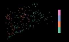
Interactions are included using the interaction operator,:. The interaction operator returns the interaction betweenvariables and is most useful when used with categorical variables. Tosummarize the interaction betweenELEV_CAT andAREA_CAT, run
summary(NE_Lakes, formula=~ELEV_CAT:AREA_CAT)#> total ELEV_CAT:AREA_CAT#> total:195 low:small :82#> high:small:53#> low:large :30#> high:large:30Levels of each variable are separated by:. For example,there are 86 lakes that are in the low elevation category and the smallarea category. To visualize this interaction, run
The formula accommodates the* operator, which combinesthe+ and: operators. For example,ELEV_CAT*AREA_CAT is shorthand forELEV_CAT + AREA_CAT + ELEV_CAT:AREA_CAT. The formula alsoaccommodates the. operator, which is shorthand for allvariables separated by+.
Two-sided formulas
Two-sided formulas are used to summarize the distribution of aleft-hand side variable for each level of each right-hand side variable.To summarize the distribution ofELEV for each level ofAREA_CAT, run
summary(NE_Lakes, formula=ELEV~AREA_CAT)#> ELEV by total:#> Min. 1st Qu. Median Mean 3rd Qu. Max.#> total 0 21.925 69.09 127.3862 203.255 561.41#>#> ELEV by AREA_CAT:#> Min. 1st Qu. Median Mean 3rd Qu. Max.#> small 0.00 19.64 59.660 117.4473 176.1700 561.41#> large 0.01 26.75 102.415 149.7487 241.2025 537.84To visualize the distribution ofELEV for each level ofAREA_CAT, run
plot(NE_Lakes, formula=ELEV~AREA_CAT)

To only summarize or visualize a particular level of a singleright-hand side variable, use theonlyshow argument:
summary(NE_Lakes, formula=ELEV~AREA_CAT, onlyshow="small")#> ELEV by AREA_CAT:#> Min. 1st Qu. Median Mean 3rd Qu. Max.#> small 0 19.64 59.66 117.4473 176.17 561.41plot(NE_Lakes, formula=ELEV~AREA_CAT, onlyshow="small")
To summarize the distribution ofELEV_CAT for each levelofAREA_CAT, run
summary(NE_Lakes, formula=ELEV_CAT~AREA_CAT)#> ELEV_CAT by total:#> low high#> total 112 83#>#> ELEV_CAT by AREA_CAT:#> low high#> small 82 53#> large 30 30To visualize the distribution ofELEV_CAT for each levelofAREA_CAT, run


Adjusting graphical parameters
There are three arguments inplot() that can adjustgraphical parameters:
var_argsadjusts graphical parameters simultaneouslyfor all levels of a variablevarlevel_argsadjusts graphical parameters uniquely foreach level of a variable...adjusts graphical parameters for simultaneously forall levels of all variables
Thevar_args andvarlevel_args argumentstake lists whose names match variable names in the formula. Forvarlevel_args, each list element must have an element namedlevels that matches the variable’s levels. The followingexample combines all three graphical parameter adjustment arguments:
list1<-list(main="Elevation Categories", pal=rainbow)list2<-list(main="Area Categories")list3<-list(levels=c("small","large"), pch=c(4,19))plot(NE_Lakes, formula=~ELEV_CAT+AREA_CAT, var_args=list(ELEV_CAT=list1, AREA_CAT=list2), varlevel_args=list(AREA_CAT=list3), cex=0.75, key.width=lcm(3))
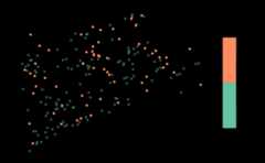
var_args useslist1 to give theELEV_CAT visualization a new title and color palette;var_args useslist2 to give theAREA_CAT visualization a new title;varlevel_args useslist3 to give theAREA_CAT visualization different shapes for the small andlarge levels;... usescex = 0.75 to reducethe size of all points; and... useskey.widthto adjust legend spacing for all visualizations.
If a two-sided formula is used, it is possible to adjust graphicalparameters of the left-hand side variable for all levels of a right-handside variable. This occurs when a sublist matching the structure ofvarlevel_args is used as an argument tovar_args. In this next example, different shapes are usedfor the small and large levels ofAREA_CAT for all levelsofELEV_CAT:
sublist<-list(AREA_CAT=list3)plot(NE_Lakes, formula=AREA_CAT~ELEV_CAT, var_args=list(ELEV_CAT=sublist), key.width=lcm(3))

Design sites
Design sites (output from thegrts() orirs() functions) can be summarized and visualized usingsummary() andplot() very similarly to howsampling frames were summarized and visualized in the previous section.Soon you will use thegrts() function to select a spatiallybalanced sample. Thegrts() function does incorporaterandomness, so to match your results with this output exactly you willneed to set a reproducible seed by running
set.seed(51)First we will obtain some design sites: To select an equalprobability GRTS sample of size 50 with 10 reverse hierarchicallyordered replacement sites, run
eqprob_rho<-grts(NE_Lakes, n_base=50, n_over=10)Similar tosummary() andplot() forsampling frames,summary() andplot() fordesign sites uses a formula. The formula should includesiteuse, which is the name of the variable in the designsites object that indicates the type of each site. The default formulaforsummary() andplot() is~siteuse, which summarizes or visualizes thesites objects in the design sites object. By default, theformula is applied to all non-NULLsitesobjects (ineqprob_rho, the nonNULL sitesobjects aresites_base (for the base sites) andsites_over (for the reverse hierarchically orderedreplacement sites)).
summary(eqprob_rho)#> total siteuse#> total:60 Base:50#> Over:10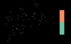
The sampling frame may be included as an argument to theplot() function:

When you includesiteuse as a left-hand side variable(siteuse is treated as a categorical variable), you cansummarize and visualize thesites object for each level ofeach right-hand side variable:
summary(eqprob_rho, formula=siteuse~AREA_CAT)#> siteuse by total:#> Base Over#> total 50 10#>#> siteuse by AREA_CAT:#> Base Over#> small 35 7#> large 15 3

You can also summarize and visualize a left-hand side variable foreach level ofsiteuse:
summary(eqprob_rho, formula=ELEV~siteuse)#> ELEV by total:#> Min. 1st Qu. Median Mean 3rd Qu. Max.#> total 0.03 26.385 65.535 135.364 214.2075 537.84#>#> ELEV by siteuse:#> Min. 1st Qu. Median Mean 3rd Qu. Max.#> Base 0.68 29.4850 81.76 148.0362 263.640 537.84#> Over 0.03 15.1275 54.49 72.0030 119.365 209.25plot(eqprob_rho, formula=ELEV~siteuse)

Analysis data
sp_summarize() andplot() work for analysisdata the same way they do for sampling frames. TheNLA_PNWanalysis data in spsurvey is analysis data (as ansfobject) from lakes in California, Oregon, and Washington. There are twovariables inNLA_PNW you will use next:
STATE: state name (California,Washington, andOregon)NITR_COND: nitrogen content categories(Poor,Fair, andGood)
Before summarizing or visualizing a sampling frame, turn it into anobject usingsp_frame():
NLA_PNW<-sp_frame(NLA_PNW)To summarize and visualizeNITR_COND across all states,run
summary(NLA_PNW, formula=~NITR_COND)#> total NITR_COND#> total:96 Fair:24#> Good:38#> Poor:34
Suppose the sampling design was stratified bySTATE. Tosummarize and visualizeNITR_COND bySTATE,run
summary(NLA_PNW, formula=NITR_COND~STATE)#> NITR_COND by total:#> Fair Good Poor#> total 24 38 34#>#> NITR_COND by STATE:#> Fair Good Poor#> California 6 8 5#> Oregon 8 26 13#> Washington 10 4 16