Note
Go to the endto download the full example code or to run this example in your browser via JupyterLite or Binder.
Lighting Properties#
Control aspects of the rendered mesh’s lighting such as Ambient, Diffuse,and Specular. These options only work if thelighting argument toadd_mesh isTrue (it’sTrue by default).
You can turn off all lighting for the given mesh by passinglighting=Falsetoadd_mesh.
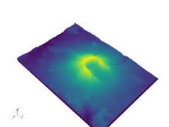
First, lets take a look at the mesh with default lighting conditions

What about with no lighting
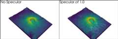
Demonstration of the specular property
p=pv.Plotter(shape=(1,2),window_size=[1500,500])p.subplot(0,0)p.add_mesh(mesh,show_scalar_bar=False)p.add_text("No Specular")p.subplot(0,1)s=1.0p.add_mesh(mesh,specular=s,show_scalar_bar=False)p.add_text(f"Specular of{s}")p.link_views()p.view_isometric()p.show(cpos=cpos)
Just specular

Specular power
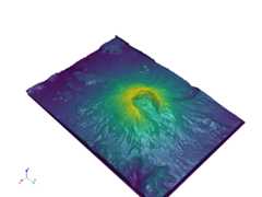
Demonstration of all three in use

Total running time of the script: (0 minutes 12.867 seconds)
Estimated memory usage: 343 MB