1.5.Stochastic Gradient Descent #

Stochastic Gradient Descent (SGD) is a simple yet very efficientapproach to fitting linear classifiers and regressors underconvex loss functions such as (linear)Support Vector Machines andLogisticRegression.Even though SGD has been around in the machine learning community fora long time, it has received a considerable amount of attention justrecently in the context of large-scale learning.

SGD has been successfully applied to large-scale and sparse machinelearning problems often encountered in text classification and naturallanguage processing. Given that the data is sparse, the classifiersin this module easily scale to problems with more than\(10^5\) trainingexamples and more than\(10^5\) features.

Strictly speaking, SGD is merely an optimization technique and does notcorrespond to a specific family of machine learning models. It is only away to train a model. Often, an instance ofSGDClassifier orSGDRegressor will have an equivalent estimator inthe scikit-learn API, potentially using a different optimization technique.For example, usingSGDClassifier(loss='log_loss') results in logistic regression,i.e. a model equivalent toLogisticRegressionwhich is fitted via SGD instead of being fitted by one of the other solversinLogisticRegression. Similarly,SGDRegressor(loss='squared_error',penalty='l2') andRidge solve the same optimization problem, viadifferent means.

The advantages of Stochastic Gradient Descent are:

Efficiency.
Ease of implementation (lots of opportunities for code tuning).

The disadvantages of Stochastic Gradient Descent include:

SGD requires a number of hyperparameters such as the regularizationparameter and the number of iterations.
SGD is sensitive to feature scaling.

Warning

Make sure you permute (shuffle) your training data before fitting the modelor useshuffle=True to shuffle after each iteration (used by default).Also, ideally, features should be standardized using e.g.make_pipeline(StandardScaler(),SGDClassifier()) (seePipelines).

1.5.1.Classification#

The classSGDClassifier implements a plain stochastic gradientdescent learning routine which supports different loss functions andpenalties for classification. Below is the decision boundary of aSGDClassifier trained with the hinge loss, equivalent to a linear SVM.

../_images/sphx_glr_plot_sgd_separating_hyperplane_001.png

As other classifiers, SGD has to be fitted with two arrays: an arrayXof shape (n_samples, n_features) holding the training samples, and anarrayy of shape (n_samples,) holding the target values (class labels)for the training samples:

>>>fromsklearn.linear_modelimportSGDClassifier>>>X=[[0.,0.],[1.,1.]]>>>y=[0,1]>>>clf=SGDClassifier(loss="hinge",penalty="l2",max_iter=5)>>>clf.fit(X,y)SGDClassifier(max_iter=5)

After being fitted, the model can then be used to predict new values:

>>>clf.predict([[2.,2.]])array([1])

SGD fits a linear model to the training data. Thecoef_ attribute holdsthe model parameters:

>>>clf.coef_array([[9.9, 9.9]])

Theintercept_ attribute holds the intercept (aka offset or bias):

>>>clf.intercept_array([-9.9])

Whether or not the model should use an intercept, i.e. a biasedhyperplane, is controlled by the parameterfit_intercept.

The signed distance to the hyperplane (computed as the dot product betweenthe coefficients and the input sample, plus the intercept) is given bySGDClassifier.decision_function:

>>>clf.decision_function([[2.,2.]])array([29.6])

The concrete loss function can be set via thelossparameter.SGDClassifier supports the following loss functions:

loss="hinge": (soft-margin) linear Support Vector Machine,
loss="modified_huber": smoothed hinge loss,
loss="log_loss": logistic regression,
and all regression losses below. In this case the target is encoded as\(-1\)or\(1\), and the problem is treated as a regression problem. The predictedclass then corresponds to the sign of the predicted target.

Please refer to themathematical section below for formulas.The first two loss functions are lazy, they only update the modelparameters if an example violates the margin constraint, which makestraining very efficient and may result in sparser models (i.e. with more zerocoefficients), even when\(L_2\) penalty is used.

Usingloss="log_loss" orloss="modified_huber" enables thepredict_proba method, which gives a vector of probability estimates\(P(y|x)\) per sample\(x\):

>>>clf=SGDClassifier(loss="log_loss",max_iter=5).fit(X,y)>>>clf.predict_proba([[1.,1.]])array([[0.00, 0.99]])

The concrete penalty can be set via thepenalty parameter.SGD supports the following penalties:

penalty="l2":\(L_2\) norm penalty oncoef_.
penalty="l1":\(L_1\) norm penalty oncoef_.
penalty="elasticnet": Convex combination of\(L_2\) and\(L_1\);(1-l1_ratio)*L2+l1_ratio*L1.

The default setting ispenalty="l2". The\(L_1\) penalty leads to sparsesolutions, driving most coefficients to zero. The Elastic Net[11] solvessome deficiencies of the\(L_1\) penalty in the presence of highly correlatedattributes. The parameterl1_ratio controls the convex combinationof\(L_1\) and\(L_2\) penalty.

SGDClassifier supports multi-class classification by combiningmultiple binary classifiers in a “one versus all” (OVA) scheme. For eachof the\(K\) classes, a binary classifier is learned that discriminatesbetween that and all other\(K-1\) classes. At testing time, we compute theconfidence score (i.e. the signed distances to the hyperplane) for eachclassifier and choose the class with the highest confidence. The Figurebelow illustrates the OVA approach on the iris dataset. The dashedlines represent the three OVA classifiers; the background colors showthe decision surface induced by the three classifiers.

../_images/sphx_glr_plot_sgd_iris_001.png

In the case of multi-class classificationcoef_ is a two-dimensionalarray of shape (n_classes, n_features) andintercept_ is aone-dimensional array of shape (n_classes,). The\(i\)-th row ofcoef_ holdsthe weight vector of the OVA classifier for the\(i\)-th class; classes areindexed in ascending order (see attributeclasses_).Note that, in principle, since they allow to create a probability model,loss="log_loss" andloss="modified_huber" are more suitable forone-vs-all classification.

SGDClassifier supports both weighted classes and weightedinstances via the fit parametersclass_weight andsample_weight. Seethe examples below and the docstring ofSGDClassifier.fit forfurther information.

SGDClassifier supports averaged SGD (ASGD)[10]. Averaging can beenabled by settingaverage=True. ASGD performs the same updates as theregular SGD (seeMathematical formulation), but instead of usingthe last value of the coefficients as thecoef_ attribute (i.e. the valuesof the last update),coef_ is set instead to theaverage value of thecoefficients across all updates. The same is done for theintercept_attribute. When using ASGD the learning rate can be larger and even constant,leading on some datasets to a speed up in training time.

For classification with a logistic loss, another variant of SGD with anaveraging strategy is available with Stochastic Average Gradient (SAG)algorithm, available as a solver inLogisticRegression.

Examples

SGD: Maximum margin separating hyperplane
Plot multi-class SGD on the iris dataset
SGD: Weighted samples
SVM: Separating hyperplane for unbalanced classes(See the Note in the example)

1.5.2.Regression#

The classSGDRegressor implements a plain stochastic gradientdescent learning routine which supports different loss functions andpenalties to fit linear regression models.SGDRegressor iswell suited for regression problems with a large number of trainingsamples (> 10.000), for other problems we recommendRidge,Lasso, orElasticNet.

The concrete loss function can be set via thelossparameter.SGDRegressor supports the following loss functions:

loss="squared_error": Ordinary least squares,
loss="huber": Huber loss for robust regression,
loss="epsilon_insensitive": linear Support Vector Regression.

Please refer to themathematical section below for formulas.The Huber and epsilon-insensitive loss functions can be used forrobust regression. The width of the insensitive region has to bespecified via the parameterepsilon. This parameter depends on thescale of the target variables.

Thepenalty parameter determines the regularization to be used (seedescription above in the classification section).

SGDRegressor also supports averaged SGD[10] (here again, seedescription above in the classification section).

For regression with a squared loss and a\(L_2\) penalty, another variant ofSGD with an averaging strategy is available with Stochastic AverageGradient (SAG) algorithm, available as a solver inRidge.

Examples

Prediction Latency

1.5.3.Online One-Class SVM#

The classsklearn.linear_model.SGDOneClassSVM implements an onlinelinear version of the One-Class SVM using a stochastic gradient descent.Combined with kernel approximation techniques,sklearn.linear_model.SGDOneClassSVM can be used to approximate thesolution of a kernelized One-Class SVM, implemented insklearn.svm.OneClassSVM, with a linear complexity in the number ofsamples. Note that the complexity of a kernelized One-Class SVM is at bestquadratic in the number of samples.sklearn.linear_model.SGDOneClassSVM is thus well suited for datasetswith a large number of training samples (over 10,000) for which the SGDvariant can be several orders of magnitude faster.

Mathematical details#

Its implementation is based on the implementation of the stochasticgradient descent. Indeed, the original optimization problem of the One-ClassSVM is given by

\[\begin{split}\begin{aligned}\min_{w, \rho, \xi} & \quad \frac{1}{2}\Vert w \Vert^2 - \rho + \frac{1}{\nu n} \sum_{i=1}^n \xi_i \\\text{s.t.} & \quad \langle w, x_i \rangle \geq \rho - \xi_i \quad 1 \leq i \leq n \\& \quad \xi_i \geq 0 \quad 1 \leq i \leq n\end{aligned}\end{split}\]

where\(\nu \in (0, 1]\) is the user-specified parameter controlling theproportion of outliers and the proportion of support vectors. Getting rid ofthe slack variables\(\xi_i\) this problem is equivalent to

\[\min_{w, \rho} \frac{1}{2}\Vert w \Vert^2 - \rho + \frac{1}{\nu n} \sum_{i=1}^n \max(0, \rho - \langle w, x_i \rangle) \, .\]

Multiplying by the constant\(\nu\) and introducing the intercept\(b = 1 - \rho\) we obtain the following equivalent optimization problem

\[\min_{w, b} \frac{\nu}{2}\Vert w \Vert^2 + b\nu + \frac{1}{n} \sum_{i=1}^n \max(0, 1 - (\langle w, x_i \rangle + b)) \, .\]

This is similar to the optimization problems studied in sectionMathematical formulation with\(y_i = 1, 1 \leq i \leq n\) and\(\alpha = \nu/2\),\(L\) being the hinge loss function and\(R\)being the\(L_2\) norm. We just need to add the term\(b\nu\) in theoptimization loop.

AsSGDClassifier andSGDRegressor,SGDOneClassSVMsupports averaged SGD. Averaging can be enabled by settingaverage=True.

Examples

One-Class SVM versus One-Class SVM using Stochastic Gradient Descent

1.5.4.Stochastic Gradient Descent for sparse data#

Note

The sparse implementation produces slightly different resultsfrom the dense implementation, due to a shrunk learning rate for theintercept. SeeImplementation details.

There is built-in support for sparse data given in any matrix in a formatsupported byscipy.sparse. For maximumefficiency, however, use the CSRmatrix format as defined inscipy.sparse.csr_matrix.

Examples

Classification of text documents using sparse features

1.5.5.Complexity#

The major advantage of SGD is its efficiency, which is basicallylinear in the number of training examples. If\(X\) is a matrix of size\(n \times p\) (with\(n\) samples and\(p\) features),training has a cost of\(O(k n \bar p)\), where\(k\) is the numberof iterations (epochs) and\(\bar p\) is the average number ofnon-zero attributes per sample.

Recent theoretical results, however, show that the runtime to get somedesired optimization accuracy does not increase as the training set size increases.

1.5.6.Stopping criterion#

The classesSGDClassifier andSGDRegressor provide twocriteria to stop the algorithm when a given level of convergence is reached:

Withearly_stopping=True, the input data is split into a training setand a validation set. The model is then fitted on the training set, and thestopping criterion is based on the prediction score (using thescoremethod) computed on the validation set. The size of the validation setcan be changed with the parametervalidation_fraction.
Withearly_stopping=False, the model is fitted on the entire input dataand the stopping criterion is based on the objective function computed onthe training data.

In both cases, the criterion is evaluated once by epoch, and the algorithm stopswhen the criterion does not improven_iter_no_change times in a row. Theimprovement is evaluated with absolute tolerancetol, and the algorithmstops in any case after a maximum number of iterationsmax_iter.

SeeEarly stopping of Stochastic Gradient Descent for anexample of the effects of early stopping.

1.5.7.Tips on Practical Use#

Stochastic Gradient Descent is sensitive to feature scaling, so itis highly recommended to scale your data. For example, scale eachattribute on the input vector\(X\) to\([0,1]\) or\([-1,1]\), or standardizeit to have mean\(0\) and variance\(1\). Note that thesame scaling must beapplied to the test vector to obtain meaningful results. This can be easilydone usingStandardScaler:
```
fromsklearn.preprocessingimportStandardScalerscaler=StandardScaler()scaler.fit(X_train)# Don't cheat - fit only on training dataX_train=scaler.transform(X_train)X_test=scaler.transform(X_test)# apply same transformation to test data# Or better yet: use a pipeline!fromsklearn.pipelineimportmake_pipelineest=make_pipeline(StandardScaler(),SGDClassifier())est.fit(X_train)est.predict(X_test)
```
If your attributes have an intrinsic scale (e.g. word frequencies orindicator features) scaling is not needed.
Finding a reasonable regularization term\(\alpha\) isbest done using automatic hyper-parameter search, e.g.GridSearchCV orRandomizedSearchCV, usually in therange10.0**-np.arange(1,7).
Empirically, we found that SGD converges after observingapproximately\(10^6\) training samples. Thus, a reasonable first guessfor the number of iterations ismax_iter=np.ceil(10**6/n),wheren is the size of the training set.
If you apply SGD to features extracted using PCA we found thatit is often wise to scale the feature values by some constantcsuch that the average\(L_2\) norm of the training data equals one.
We found that Averaged SGD works best with a larger number of featuresand a highereta0.

References

“Efficient BackProp”Y. LeCun, L. Bottou, G. Orr, K. Müller - In Neural Networks: Tricksof the Trade 1998.

1.5.8.Mathematical formulation#

We describe here the mathematical details of the SGD procedure. A goodoverview with convergence rates can be found in[12].

Given a set of training examples\(\{(x_1, y_1), \ldots, (x_n, y_n)\}\) where\(x_i \in \mathbf{R}^m\) and\(y_i \in \mathbf{R}\)(\(y_i \in \{-1, 1\}\) for classification),our goal is to learn a linear scoring function\(f(x) = w^T x + b\) with model parameters\(w \in \mathbf{R}^m\) andintercept\(b \in \mathbf{R}\). In order to make predictions for binaryclassification, we simply look at the sign of\(f(x)\). To find the modelparameters, we minimize the regularized training error given by

\[E(w,b) = \frac{1}{n}\sum_{i=1}^{n} L(y_i, f(x_i)) + \alpha R(w)\]

where\(L\) is a loss function that measures model (mis)fit and\(R\) is a regularization term (aka penalty) that penalizes modelcomplexity;\(\alpha > 0\) is a non-negative hyperparameter that controlsthe regularization strength.

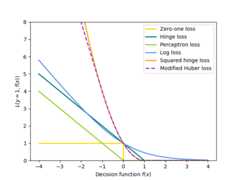
Loss functions details#

Different choices for\(L\) entail different classifiers or regressors:

Hinge (soft-margin): equivalent to Support Vector Classification.\(L(y_i, f(x_i)) = \max(0, 1 - y_i f(x_i))\).
Perceptron:\(L(y_i, f(x_i)) = \max(0, - y_i f(x_i))\).
Modified Huber:\(L(y_i, f(x_i)) = \max(0, 1 - y_i f(x_i))^2\) if\(y_i f(x_i) >-1\), and\(L(y_i, f(x_i)) = -4 y_i f(x_i)\) otherwise.
Log Loss: equivalent to Logistic Regression.\(L(y_i, f(x_i)) = \log(1 + \exp (-y_i f(x_i)))\).
Squared Error: Linear regression (Ridge or Lasso depending on\(R\)).\(L(y_i, f(x_i)) = \frac{1}{2}(y_i - f(x_i))^2\).
Huber: less sensitive to outliers than least-squares. It is equivalent toleast squares when\(|y_i - f(x_i)| \leq \varepsilon\), and\(L(y_i, f(x_i)) = \varepsilon |y_i - f(x_i)| - \frac{1}{2}\varepsilon^2\) otherwise.
Epsilon-Insensitive: (soft-margin) equivalent to Support Vector Regression.\(L(y_i, f(x_i)) = \max(0, |y_i - f(x_i)| - \varepsilon)\).

All of the above loss functions can be regarded as an upper bound on themisclassification error (Zero-one loss) as shown in the Figure below.

../_images/sphx_glr_plot_sgd_loss_functions_001.png

Popular choices for the regularization term\(R\) (thepenaltyparameter) include:

\(L_2\) norm:\(R(w) := \frac{1}{2} \sum_{j=1}^{m} w_j^2 = ||w||_2^2\),
\(L_1\) norm:\(R(w) := \sum_{j=1}^{m} |w_j|\), which leads to sparsesolutions.
Elastic Net:\(R(w) := \frac{\rho}{2} \sum_{j=1}^{n} w_j^2 +(1-\rho) \sum_{j=1}^{m} |w_j|\), a convex combination of\(L_2\) and\(L_1\), where\(\rho\) is given by1-l1_ratio.

The Figure below shows the contours of the different regularization termsin a 2-dimensional parameter space (\(m=2\)) when\(R(w) = 1\).

../_images/sphx_glr_plot_sgd_penalties_001.png

1.5.8.1.SGD#

Stochastic gradient descent is an optimization method for unconstrainedoptimization problems. In contrast to (batch) gradient descent, SGDapproximates the true gradient of\(E(w,b)\) by considering asingle training example at a time.

The classSGDClassifier implements a first-order SGD learningroutine. The algorithm iterates over the training examples and for eachexample updates the model parameters according to the update rule given by

\[w \leftarrow w - \eta \left[\alpha \frac{\partial R(w)}{\partial w}+ \frac{\partial L(w^T x_i + b, y_i)}{\partial w}\right]\]

where\(\eta\) is the learning rate which controls the step-size inthe parameter space. The intercept\(b\) is updated similarly butwithout regularization (and with additional decay for sparse matrices, asdetailed inImplementation details).

The learning rate\(\eta\) can be either constant or gradually decaying. Forclassification, the default learning rate schedule (learning_rate='optimal')is given by

\[\eta^{(t)} = \frac {1}{\alpha (t_0 + t)}\]

where\(t\) is the time step (there are a total ofn_samples*n_itertime steps),\(t_0\) is determined based on a heuristic proposed by Léon Bottousuch that the expected initial updates are comparable with the expectedsize of the weights (this assumes that the norm of the training samples isapproximately 1). The exact definition can be found in_init_t inBaseSGD.

For regression the default learning rate schedule is inverse scaling(learning_rate='invscaling'), given by

\[\eta^{(t)} = \frac{\eta_0}{t^{power\_t}}\]

where\(\eta_0\) and\(power\_t\) are hyperparameters chosen by theuser viaeta0 andpower_t, respectively.

For a constant learning rate uselearning_rate='constant' and useeta0to specify the learning rate.

For an adaptively decreasing learning rate, uselearning_rate='adaptive'and useeta0 to specify the starting learning rate. When the stoppingcriterion is reached, the learning rate is divided by 5, and the algorithmdoes not stop. The algorithm stops when the learning rate goes below1e-6.

The model parameters can be accessed through thecoef_ andintercept_ attributes:coef_ holds the weights\(w\) andintercept_ holds\(b\).

When using Averaged SGD (with theaverage parameter),coef_ is set to theaverage weight across all updates:coef_\(= \frac{1}{T} \sum_{t=0}^{T-1} w^{(t)}\),where\(T\) is the total number of updates, found in thet_ attribute.

1.5.9.Implementation details#

The implementation of SGD is influenced by theStochasticGradientSVM of[7].Similar to SvmSGD,the weight vector is represented as the product of a scalar and a vectorwhich allows an efficient weight update in the case of\(L_2\) regularization.In the case of sparse inputX, the intercept is updated with asmaller learning rate (multiplied by 0.01) to account for the fact thatit is updated more frequently. Training examples are picked up sequentiallyand the learning rate is lowered after each observed example. We adopted thelearning rate schedule from[8].For multi-class classification, a “one versus all” approach is used.We use the truncated gradient algorithm proposed in[9]for\(L_1\) regularization (and the Elastic Net).The code is written in Cython.

References

[7]“Stochastic Gradient Descent” L. Bottou - Website, 2010.
[8]“Pegasos: Primal estimated sub-gradient solver for svm”S. Shalev-Shwartz, Y. Singer, N. Srebro - In Proceedings of ICML ‘07.
[9]“Stochastic gradient descent training for l1-regularizedlog-linear models with cumulative penalty”Y. Tsuruoka, J. Tsujii, S. Ananiadou - In Proceedings of the AFNLP/ACL’09.
[10](1,2)“Towards Optimal One Pass Large Scale Learning withAveraged Stochastic Gradient Descent”. Xu, Wei (2011)
[11]“Regularization and variable selection via the elastic net”H. Zou, T. Hastie - Journal of the Royal Statistical Society Series B,67 (2), 301-320.
[12]“Solving large scale linear prediction problems using stochasticgradient descent algorithms”T. Zhang - In Proceedings of ICML ‘04.