
Note
Go to the endto download the full example code or to run this example in your browser via Binder.
Using Polar and Log-Polar Transformations for Registration#
Phase correlation (registration.phase_cross_correlation) is an efficientmethod for determining translation offset between pairs of similar images.However this approach relies on a near absence of rotation/scaling differencesbetween the images, which are typical in real-world examples.
To recover rotation and scaling differences between two images, we can takeadvantage of two geometric properties of the log-polar transform and thetranslation invariance of the frequency domain. First, rotation in Cartesianspace becomes translation along the angular coordinate (\(\theta\)) axisof log-polar space. Second, scaling in Cartesian space becomes translationalong the radial coordinate (\(\rho = \ln\sqrt{x^2 + y^2}\)) of log-polarspace. Finally, differences in translation in the spatial domain do not impactmagnitude spectrum in the frequency domain.
In this series of examples, we build on these concepts to show how thelog-polar transformtransform.warp_polar can be used in conjunction withphase correlation to recover rotation and scaling differences between twoimages that also have a translation offset.
Recover rotation difference with a polar transform#
In this first example, we consider the simple case of two images that onlydiffer with respect to rotation around a common center point. By remappingthese images into polar space, the rotation difference becomes a simpletranslation difference that can be recovered by phase correlation.
importnumpyasnpimportmatplotlib.pyplotaspltfromskimageimportdatafromskimage.registrationimportphase_cross_correlationfromskimage.transformimportwarp_polar,rotate,rescalefromskimage.utilimportimg_as_floatradius=705angle=35image=data.retina()image=img_as_float(image)rotated=rotate(image,angle)image_polar=warp_polar(image,radius=radius,channel_axis=-1)rotated_polar=warp_polar(rotated,radius=radius,channel_axis=-1)fig,axes=plt.subplots(2,2,figsize=(8,8))ax=axes.ravel()ax[0].set_title("Original")ax[0].imshow(image)ax[1].set_title("Rotated")ax[1].imshow(rotated)ax[2].set_title("Polar-Transformed Original")ax[2].imshow(image_polar)ax[3].set_title("Polar-Transformed Rotated")ax[3].imshow(rotated_polar)plt.show()shifts,error,phasediff=phase_cross_correlation(image_polar,rotated_polar,normalization=None)print(f'Expected value for counterclockwise rotation in degrees: 'f'{angle}')print(f'Recovered value for counterclockwise rotation: 'f'{shifts[0]}')

Expected value for counterclockwise rotation in degrees: 35Recovered value for counterclockwise rotation: 35.0
Recover rotation and scaling differences with log-polar transform#
In this second example, the images differ by both rotation and scaling (notethe axis tick values). By remapping these images into log-polar space,we can recover rotation as before, and now also scaling, by phasecorrelation.
# radius must be large enough to capture useful info in larger imageradius=1500angle=53.7scale=2.2image=data.retina()image=img_as_float(image)rotated=rotate(image,angle)rescaled=rescale(rotated,scale,channel_axis=-1)image_polar=warp_polar(image,radius=radius,scaling='log',channel_axis=-1)rescaled_polar=warp_polar(rescaled,radius=radius,scaling='log',channel_axis=-1)fig,axes=plt.subplots(2,2,figsize=(8,8))ax=axes.ravel()ax[0].set_title("Original")ax[0].imshow(image)ax[1].set_title("Rotated and Rescaled")ax[1].imshow(rescaled)ax[2].set_title("Log-Polar-Transformed Original")ax[2].imshow(image_polar)ax[3].set_title("Log-Polar-Transformed Rotated and Rescaled")ax[3].imshow(rescaled_polar)plt.show()# setting `upsample_factor` can increase precisionshifts,error,phasediff=phase_cross_correlation(image_polar,rescaled_polar,upsample_factor=20,normalization=None)shiftr,shiftc=shifts[:2]# Calculate scale factor from translationklog=radius/np.log(radius)shift_scale=1/(np.exp(shiftc/klog))print(f'Expected value for cc rotation in degrees:{angle}')print(f'Recovered value for cc rotation:{shiftr}')print()print(f'Expected value for scaling difference:{scale}')print(f'Recovered value for scaling difference:{shift_scale}')
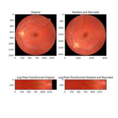
Expected value for cc rotation in degrees: 53.7Recovered value for cc rotation: 53.75Expected value for scaling difference: 2.2Recovered value for scaling difference: 2.1981889915232165
Register rotation and scaling on a translated image - Part 1#
The above examples only work when the images to be registered share acenter. However, it is more often the case that there is also a translationcomponent to the difference between two images to be registered. Oneapproach to register rotation, scaling and translation is to first correctfor rotation and scaling, then solve for translation. It is possible toresolve rotation and scaling differences for translated images by working onthe magnitude spectra of the Fourier-transformed images.
In this next example, we first show how the above approaches fail when twoimages differ by rotation, scaling, and translation.
fromskimage.colorimportrgb2grayfromskimage.filtersimportwindow,difference_of_gaussiansfromscipy.fftimportfft2,fftshiftangle=24scale=1.4shiftr=30shiftc=15image=rgb2gray(data.retina())translated=image[shiftr:,shiftc:]rotated=rotate(translated,angle)rescaled=rescale(rotated,scale)sizer,sizec=image.shaperts_image=rescaled[:sizer,:sizec]# When center is not shared, log-polar transform is not helpful!radius=705warped_image=warp_polar(image,radius=radius,scaling="log")warped_rts=warp_polar(rts_image,radius=radius,scaling="log")shifts,error,phasediff=phase_cross_correlation(warped_image,warped_rts,upsample_factor=20,normalization=None)shiftr,shiftc=shifts[:2]klog=radius/np.log(radius)shift_scale=1/(np.exp(shiftc/klog))fig,axes=plt.subplots(2,2,figsize=(8,8))ax=axes.ravel()ax[0].set_title("Original Image")ax[0].imshow(image,cmap='gray')ax[1].set_title("Modified Image")ax[1].imshow(rts_image,cmap='gray')ax[2].set_title("Log-Polar-Transformed Original")ax[2].imshow(warped_image)ax[3].set_title("Log-Polar-Transformed Modified")ax[3].imshow(warped_rts)fig.suptitle('log-polar-based registration fails when no shared center')plt.show()print(f'Expected value for cc rotation in degrees:{angle}')print(f'Recovered value for cc rotation:{shiftr}')print()print(f'Expected value for scaling difference:{scale}')print(f'Recovered value for scaling difference:{shift_scale}')

Expected value for cc rotation in degrees: 24Recovered value for cc rotation: -167.55Expected value for scaling difference: 1.4Recovered value for scaling difference: 25.110458986143573
Register rotation and scaling on a translated image - Part 2#
We next show how rotation and scaling differences, but not translationdifferences, are apparent in the frequency magnitude spectra of the images.These differences can be recovered by treating the magnitude spectra asimages themselves, and applying the same log-polar + phase correlationapproach taken above.
# First, band-pass filter both imagesimage=difference_of_gaussians(image,5,20)rts_image=difference_of_gaussians(rts_image,5,20)# window imageswimage=image*window('hann',image.shape)rts_wimage=rts_image*window('hann',image.shape)# work with shifted FFT magnitudesimage_fs=np.abs(fftshift(fft2(wimage)))rts_fs=np.abs(fftshift(fft2(rts_wimage)))# Create log-polar transformed FFT mag images and registershape=image_fs.shaperadius=shape[0]//8# only take lower frequencieswarped_image_fs=warp_polar(image_fs,radius=radius,output_shape=shape,scaling='log',order=0)warped_rts_fs=warp_polar(rts_fs,radius=radius,output_shape=shape,scaling='log',order=0)warped_image_fs=warped_image_fs[:shape[0]//2,:]# only use half of FFTwarped_rts_fs=warped_rts_fs[:shape[0]//2,:]shifts,error,phasediff=phase_cross_correlation(warped_image_fs,warped_rts_fs,upsample_factor=10,normalization=None)# Use translation parameters to calculate rotation and scaling parametersshiftr,shiftc=shifts[:2]recovered_angle=(360/shape[0])*shiftrklog=shape[1]/np.log(radius)shift_scale=np.exp(shiftc/klog)fig,axes=plt.subplots(2,2,figsize=(8,8))ax=axes.ravel()ax[0].set_title("Original Image FFT\n(magnitude; zoomed)")center=np.array(shape)//2ax[0].imshow(image_fs[center[0]-radius:center[0]+radius,center[1]-radius:center[1]+radius],cmap='magma',)ax[1].set_title("Modified Image FFT\n(magnitude; zoomed)")ax[1].imshow(rts_fs[center[0]-radius:center[0]+radius,center[1]-radius:center[1]+radius],cmap='magma',)ax[2].set_title("Log-Polar-Transformed\nOriginal FFT")ax[2].imshow(warped_image_fs,cmap='magma')ax[3].set_title("Log-Polar-Transformed\nModified FFT")ax[3].imshow(warped_rts_fs,cmap='magma')fig.suptitle('Working in frequency domain can recover rotation and scaling')plt.show()print(f'Expected value for cc rotation in degrees:{angle}')print(f'Recovered value for cc rotation:{recovered_angle}')print()print(f'Expected value for scaling difference:{scale}')print(f'Recovered value for scaling difference:{shift_scale}')
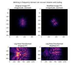
Expected value for cc rotation in degrees: 24Recovered value for cc rotation: 23.753366406803682Expected value for scaling difference: 1.4Recovered value for scaling difference: 1.3901762721757436
Some notes on this approach#
It should be noted that this approach relies on a couple of parametersthat have to be chosen ahead of time, and for which there are no clearlyoptimal choices:
1. The images should have some degree of bandpass filteringapplied, particularly to remove high frequencies, and different choices heremay impact outcome. The bandpass filter also complicates matters because,since the images to be registered will differ in scale and these scaledifferences are unknown, any bandpass filter will necessarily attenuatedifferent features between the images. For example, the log-polar transformedmagnitude spectra don’t really look “alike” in the last example here. Yet ifyou look closely, there are some common patterns in those spectra, and theydo end up aligning well by phase correlation as demonstrated.
2. Images must be windowed using windows with circular symmetry, to removethe spectral leakage coming from image borders. There is no clearly optimalchoice of window.
Finally, we note that large changes in scale will dramatically alter themagnitude spectra, especially since a big change in scale will usually beaccompanied by some cropping and loss of information content. The literatureadvises staying within 1.8-2x scale change[1][2]. This is fine for mostbiological imaging applications.
References#
[1]B.S. Reddy and B.N. Chatterji. An FFT-based technique for translation,rotation and scale- invariant image registration. IEEE Trans. ImageProcessing, 5(8):1266–1271, 1996.DOI:10.1109/83.506761
[2]Tzimiropoulos, Georgios, and Tania Stathaki. “Robust FFT-basedscale-invariant image registration.” In 4th SEAS DTC TechnicalConference. 2009.DOI:10.1109/TPAMI.2010.107
Total running time of the script: (0 minutes 7.759 seconds)