Movatterモバイル変換


[0]ホーム

URL:


Skip to main page content
U.S. flag

An official website of the United States government

Dot gov

The .gov means it’s official.
Federal government websites often end in .gov or .mil. Before sharing sensitive information, make sure you’re on a federal government site.

Https

The site is secure.
Thehttps:// ensures that you are connecting to the official website and that any information you provide is encrypted and transmitted securely.

NIH NLM Logo
Log inShow account info
Access keysNCBI HomepageMyNCBI HomepageMain ContentMain Navigation
pubmed logo
Advanced Clipboard
User Guide

Full text links

eLife Sciences Publications, Ltd full text link eLife Sciences Publications, Ltd Free PMC article
Full text links

Actions

Share

.2022 Dec 20:11:e73767.
doi: 10.7554/eLife.73767.

Modeling the spatiotemporal spread of beneficial alleles using ancient genomes

Affiliations

Modeling the spatiotemporal spread of beneficial alleles using ancient genomes

Rasa A Muktupavela et al. Elife..

Abstract

Ancient genome sequencing technologies now provide the opportunity to study natural selection in unprecedented detail. Rather than making inferences from indirect footprints left by selection in present-day genomes, we can directly observe whether a given allele was present or absent in a particular region of the world at almost any period of human history within the last 10,000 years. Methods for studying selection using ancient genomes often rely on partitioning individuals into discrete time periods or regions of the world. However, a complete understanding of natural selection requires more nuanced statistical methods which can explicitly model allele frequency changes in a continuum across space and time. Here we introduce a method for inferring the spread of a beneficial allele across a landscape using two-dimensional partial differential equations. Unlike previous approaches, our framework can handle time-stamped ancient samples, as well as genotype likelihoods and pseudohaploid sequences from low-coverage genomes. We apply the method to a panel of published ancient West Eurasian genomes to produce dynamic maps showcasing the inferred spread of candidate beneficial alleles over time and space. We also provide estimates for the strength of selection and diffusion rate for each of these alleles. Finally, we highlight possible avenues of improvement for accurately tracing the spread of beneficial alleles in more complex scenarios.

Keywords: ancient DNA; diffusion; evolution; evolutionary biology; human; lactase persistence; natural selection; spatiotemporal inference.

Plain language summary

Analyzing the genomes of our ancient ancestors can reveal how certain traits spread through the human population over the course of evolution. Mutations that make individuals better equipped to survive their environment are more likely to be passed on to the next generation and become more common. For example, a genetic variant that enables adult people to digest sugars in dairy products has become more common in humans over time. Yet evolution does not only happen across time: it transverses space as well. Modeling the geographic spread of such genetic mutations is challenging using existing methods. To overcome this, Muktupavela et al. developed a new computational method that uses modern and ancient human genomes to study the evolution of specific genetic variants across space and time. The tool can determine where certain variants first emerged, how quickly they spread across geographic areas, and how rapidly they became prevalent in human populations. Muktupavela et al. applied their new method, which was based on a previously published framework, to track the spread of two common genetic variations that have previously been reported to be subject to natural selection: one that allows adult humans to digest dairy products, and another associated with skin pigmentation. They found that the mutation that enabled dairy consumption originated around what is now southwestern Russia or eastern Ukraine. The variation then spread westward, becoming increasingly more common over the course of the Holocene. The mutation related to skin pigmentation emerged further south than the dairy-related variation, and then also spread westward. Massive human migrations during the Neolithic and Bronze Age eras may have helped disperse both variants. The model developed by Muktupavela et al. could help scientists track the geographic spread of other genetic variants in human populations, as well as provide new insights into how humans adapt to changing environmental conditions. Incorporating major events into the model, like mass migrations or glacial retreats, may lead to even more insights.

© 2022, Muktupavela et al.


Conflict of interest statement

RM, MP, LS, TK, JN, FR No competing interests declared

Figures

Figure 1.
Figure 1.. Comparison of true and inferred allele frequency dynamics for simulation B5.
(a) Comparison of true and inferred allele frequency dynamics for a simulation with diffusion and no advection (B5). The green dot corresponds to the origin of the allele. The parameter values used to generate the frequency surface maps are summarized in Appendix 2—table 1. (b) Comparison of true parameter values and model estimates. Whiskers represent 95% confidence intervals.
Figure 1—figure supplement 1.
Figure 1—figure supplement 1.. Comparison of true and inferred allele frequency dynamics for simulation B1.
(a) Comparison of true and inferred allele frequency dynamics for simulation B1. The green dot corresponds to the origin of the allele. The parameter values used to generate the frequency surface maps are summarized in Appendix 2—table 1. (b) Comparison of true parameter values and model estimates. Whiskers represent 95% confidence intervals.
Figure 1—figure supplement 2.
Figure 1—figure supplement 2.. Comparison of true and inferred allele frequency dynamics for simulation B2.
(a) Comparison of true and inferred allele frequency dynamics for simulation B2. The green dot corresponds to the origin of the allele. The parameter values used to generate the frequency surface maps are summarized in Appendix 2—table 1. (b) Comparison of true parameter values and model estimates. Whiskers represent 95% confidence intervals.
Figure 1—figure supplement 3.
Figure 1—figure supplement 3.. Comparison of true and inferred allele frequency dynamics for simulation B3.
(a) Comparison of true and inferred allele frequency dynamics for simulation B3. The green dot corresponds to the origin of the allele. The parameter values used to generate the frequency surface maps are summarized in Appendix 2—table 1. (b) Comparison of true parameter values and model estimates. Whiskers represent 95% confidence intervals.
Figure 1—figure supplement 4.
Figure 1—figure supplement 4.. Comparison of true and inferred allele frequency dynamics for simulation B4.
(a) Comparison of true and inferred allele frequency dynamics for simulation B4. The green dot corresponds to the origin of the allele. The parameter values used to generate the frequency surface maps are summarized in Appendix 2—table 1. (b) Comparison of true parameter values and model estimates. Whiskers represent 95% confidence intervals.
Figure 1—figure supplement 5.
Figure 1—figure supplement 5.. Comparison of true and inferred allele frequency dynamics for simulation B6.
(a) Comparison of true and inferred allele frequency dynamics for simulation B6. The green dot corresponds to the origin of the allele. The parameter values used to generate the frequency surface maps are summarized in Appendix 2—table 1. (b) Comparison of true parameter values and model estimates. Whiskers represent 95% confidence intervals.
Figure 1—figure supplement 6.
Figure 1—figure supplement 6.. Comparison of true allele frequency dynamics for simulation B1 and those inferred by the model C.
(a) Comparison of true allele frequency dynamics for simulation B1 and those inferred by the model C. The green dot shows the origin of the derived allele and the cross represents the location of the first individual that carried it. (b) Comparison of true parameter values and model estimates. Whiskers represent 95% confidence intervals.
Figure 1—figure supplement 7.
Figure 1—figure supplement 7.. Comparison of true allele frequency dynamics for simulation B4 and those inferred by the model C.
(a) Comparison of true allele frequency dynamics for simulation B4 and those inferred by the model C. The green dot corresponds to the origin of the allele, and the cross represents the first sample having the derived variant. (b) Comparison of true parameter values and model estimates. Whiskers represent 95% confidence intervals.
Figure 2.
Figure 2.. Comparison of true and inferred allele frequency dynamics for simulation C4.
(a) Comparison of true and inferred allele frequency dynamics for one of the simulations including advection (C4). The green dot corresponds to the origin of the allele. The parameter values used to generate the frequency surface maps are summarized in Appendix 2—table 2. (b) Comparison of true parameter values and model estimates. Whiskers represent 95% confidence intervals.
Figure 2—figure supplement 1.
Figure 2—figure supplement 1.. Comparison of true and inferred allele frequency dynamics for simulation C1.
(a) Comparison of true and inferred allele frequency dynamics for one of the simulations including advection (C1). The green dot corresponds to the origin of the allele. The parameter values used to generate the frequency surface maps are summarized in Appendix 2—table 2. (b) Comparison of true parameter values and model estimates. Whiskers represent 95% confidence intervals.
Figure 2—figure supplement 2.
Figure 2—figure supplement 2.. Comparison of true and inferred allele frequency dynamics for simulation C2.
(a) Comparison of true and inferred allele frequency dynamics for one of the simulations including advection (C2). The green dot corresponds to the origin of the allele. The parameter values used to generate the frequency surface maps are summarized in Appendix 2—table 2. (b) Comparison of true parameter values and model estimates. Whiskers represent 95% confidence intervals.
Figure 2—figure supplement 3.
Figure 2—figure supplement 3.. Comparison of true and inferred allele frequency dynamics for simulation C3.
(a) Comparison of true and inferred allele frequency dynamics for one of the simulations including advection (C3). The green dot corresponds to the origin of the allele. The parameter values used to generate the frequency surface maps are summarized in Appendix 2—table 2. (b) Comparison of true parameter values and model estimates. Whiskers represent 95% confidence intervals.
Figure 3.
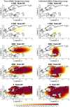
Figure 3.. Comparison of true allele frequency map and map generated using ‘intermediate 75%/25%’ clustering scheme.
Left: allele frequency map generated using true parameter values. Right: allele frequency map generated using parameter estimates for ‘intermediate 75%/25%’ clustering scheme. Parameter values used to generate the maps are summarized in Appendix 2—table 3.
Figure 3—figure supplement 1.
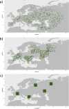
Figure 3—figure supplement 1.. Examples of spatial sampling scenarios for each of the three clustering schemes.
We chose five locations and increasingly restricted the area where we allowed the individuals to be sampled. (a) Map showing homogeneous sampling scheme in which we did not impose any spatial restrictions of individuals sampled. (b) Intermediate sampling scheme with the region restricted to 7° in each cardinal direction from each of the chosen locations. (c) Extreme sampling scheme with the sampling region restricted to 2° in each cardinal direction from the chosen locations.
Figure 3—figure supplement 2.
Figure 3—figure supplement 2.. Allele frequency map generated using true parameter values and using parameter estimates for ‘homogeneous 75%/25%’ clustering scheme.
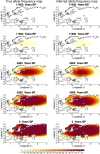
Left: allele frequency map generated using true parameter values. Right: allele frequency map generated using parameter estimates for ‘homogeneous 75%/25%’ clustering scheme. Parameter values used to generate the maps are summarized in Appendix 2—table 3.
Figure 3—figure supplement 3.
Figure 3—figure supplement 3.. Allele frequency map generated using true parameter values and using parameter estimates for ‘homogeneous 50%/50%’ clustering scheme.
Left: allele frequency map generated using true parameter values. Right: allele frequency map generated using parameter estimates for ‘homogeneous 50%/50%’ clustering scheme. Parameter values used to generate the maps are summarized in Appendix 2—table 3.
Figure 3—figure supplement 4.
Figure 3—figure supplement 4.. Allele frequency map generated using true parameter values and using parameter estimates for ‘homogeneous 25%/75%’ clustering scheme.
Left: allele frequency map generated using true parameter values. Right: allele frequency map generated using parameter estimates for ‘homogeneous 25%/75%’ clustering scheme. Parameter values used to generate the maps are summarized in Appendix 2—table 3.
Figure 3—figure supplement 5.
Figure 3—figure supplement 5.. Allele frequency map generated using true parameter values and using parameter estimates for ‘intermediate 50%/50%’ clustering scheme.
Left: allele frequency map generated using true parameter values. Right: allele frequency map generated using parameter estimates for ‘intermediate 50%/50%’ clustering scheme. Parameter values used to generate the maps are summarzsed in Appendix 2—table 3.
Figure 3—figure supplement 6.
Figure 3—figure supplement 6.. Allele frequency map generated using true parameter values and using parameter estimates for ‘intermediate 25%/75%’ clustering scheme.
Left: allele frequency map generated using true parameter values. Right: allele frequency map generated using parameter estimates for ‘intermediate 25%/75%’ clustering scheme. Parameter values used to generate the maps are summarized in Appendix 2—table 3.
Figure 3—figure supplement 7.
Figure 3—figure supplement 7.. Allele frequency map generated using true parameter values and using parameter estimates for ‘extreme 75%/25%’ clustering scheme.
Left: allele frequency map generated using true parameter values. Right: allele frequency map generated using parameter estimates for ‘extreme 75%/25%’ clustering scheme. Parameter values used to generate the maps are summarzsed in Appendix 2—table 3.
Figure 3—figure supplement 8.
Figure 3—figure supplement 8.. Allele frequency map generated using true parameter values and using parameter estimates for ‘extreme 50%/50%’ clustering scheme.
Left: allele frequency map generated using true parameter values. Right: allele frequency map generated using parameter estimates for ‘extreme 50%/50%’ clustering scheme. Parameter values used to generate the maps are summarized in Appendix 2—table 3.
Figure 3—figure supplement 9.
Figure 3—figure supplement 9.. Allele frequency map generated using true parameter values and using parameter estimates for ‘extreme 25%/75%’ clustering scheme.
Left: allele frequency map generated using true parameter values. Right: allele frequency map generated using parameter estimates for ‘extreme 25%/75%’ clustering scheme. Parameter values used to generate the maps are summarized in Appendix 2—table 3.
Figure 4.
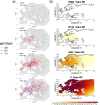
Figure 4.. Comparison of an individual-based simulation and allele frequency dynamics inferred by the diffusion model.
(A) Individual-based simulation of an allele that arose in Central Europe 15,000 years ago with a selection coefficient of 0.03. Each dot represents a genotype from a simulated genome. To avoid overplotting, only 1000 out of the total 20,000 individuals in the simulation in each time point are shown for each genotype category. (B) Allele frequency dynamics inferred by the diffusion model on the individual-based simulation to the left, after randomly sampling 1040 individuals from the simulation and performing pseudohaploid genotype sampling on them. The ages of sampled individuals were log-uniformly distributed. The estimated parameter values of the fitted model are shown in Appendix 2—table 4.
Figure 4—figure supplement 1.
Figure 4—figure supplement 1.. Distribution of individuals across the map under neutrality, showing the tendency of individuals to cluster together.
Figure 5.
Figure 5.. Locations of samples used to model the spread of the rs4988235(T) allele.
The upper panel shows the spatiotemporal locations of ancient individuals, and the bottom panel represents the locations of present-day individuals.
Figure 6.
Figure 6.. Allele frequency dynamics of rs4988235(T).
(a) Top: pseudohaploid genotypes of ancient samples at the rs4988235 SNP in different periods. Yellow corresponds to the rs4988235(T) allele. Bottom: allele frequencies of present-day samples represented as pie charts. The size of the pie charts corresponds to the number of available sequences in each region. (b) Inferred allele frequency dynamics of rs4988235(T). The green dot indicates the inferred geographic origin of the allele.
Figure 6—figure supplement 1.
Figure 6—figure supplement 1.. Inferred frequency dynamics of rs4988235(T) using the allele age that was inferred in Albers and McVean, 2020.
Figure 6—figure supplement 2.
Figure 6—figure supplement 2.. Inferred frequency dynamics of rs4988235(T) when the origin of the allele is moved 10° west from the original estimate.
Figure 6—figure supplement 3.
Figure 6—figure supplement 3.. Inferred frequency dynamics of rs4988235(T) when the origin of the allele is moved 10° east from the original estimate.
Figure 6—figure supplement 4.
Figure 6—figure supplement 4.. Inferred frequency dynamics of rs4988235(T) when the origin of the allele is moved 10° north from the original estimate.
.
Figure 6—figure supplement 5.
Figure 6—figure supplement 5.. Inferred frequency dynamics of rs4988235(T) when the origin of the allele is moved 10° south from the original estimate.
Figure 6—figure supplement 6.
Figure 6—figure supplement 6.. Inferred frequency dynamics of rs4988235(T) forcing the geographic origin of the allele to be at the location inferred in Itan et al., 2009.
Figure 6—figure supplement 7.
Figure 6—figure supplement 7.. Inferred frequency dynamics of rs4988235(T) assuming the allele age to be the lower end of the 95% credible interval for the start of selection onset inferred in Itan et al., 2009.
Figure 6—figure supplement 8.
Figure 6—figure supplement 8.. Inferred frequency dynamics of rs4988235(T) assuming the allele age to be the higher end of the 95% credible interval for the start of selection onset inferred in Itan et al., 2009.
Figure 6—figure supplement 9.
Figure 6—figure supplement 9.. Log-likelihood values for model runs using different ages of the rs4988235(T) allele as input, with the age inferred by Itan et al., 2009 we use as fixed input highlighted in red.
Figure 7.
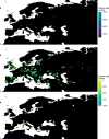
Figure 7.. Spatiotemporal sampling locations of sequences used to model the rs1042602(A) allele in Western Eurasia.
Upper panel: ancient individuals dated as older than 10,000 years ago. Middle panel: ancient individuals dated as younger than 10,000 years ago. Bottom panel: present-day individuals from the Human Genome Diversity Panel (HGDP).
Figure 8.
Figure 8.. Allele frequency dynamics of rs1042602(A).
(a) Top: pseudohaploid genotypes of ancient samples of the rs1042602 in different periods. Yellow corresponds to the A allele. Bottom: diploid genotypes of present-day samples. (b) Inferred allele frequency dynamics of rs1042602(A). The green dot corresponds to the inferred geographic origin of the allele.
Figure 8—figure supplement 1.
Figure 8—figure supplement 1.. Inferred frequency dynamics of rs1042602(A) when the origin of the allele is moved 10° east from the original estimate.
Figure 8—figure supplement 2.
Figure 8—figure supplement 2.. Inferred frequency dynamics of rs1042602(A) when the origin of the allele is moved 10° north from the original estimate.
Figure 8—figure supplement 3.
Figure 8—figure supplement 3.. Inferred frequency dynamics of rs1042602(A) when the origin of the allele is moved 10° south from the original estimate.
Figure 8—figure supplement 4.
Figure 8—figure supplement 4.. Inferred frequency dynamics of rs1042602(A) assuming the allele age to be the lower end of the 95% confidence interval for the allele age inferred in Albers and McVean, 2020.
Figure 8—figure supplement 5.
Figure 8—figure supplement 5.. Frequency dynamics of rs1042602(A) assuming the allele age to be the higher end of the 95% confidence interval for the allele age inferred in Albers and McVean, 2020.
Figure 8—figure supplement 6.
Figure 8—figure supplement 6.. Log-likelihood values for model runs using different ages of the rs1042602(A) allele as input, with the age inferred by Albers and McVean, 2020 we use as fixed input highlighted in red.
Appendix 2—figure 1.
Appendix 2—figure 1.. Maps showing areas where diffusion in the model is allowed (green) and where it is forbidden (blue).
(a) Map without land bridges. (b) Map containing land bridges indicated with red circles.
Appendix 2—figure 2.
Appendix 2—figure 2.. Geographic locations for points used as potential origins of the allele at the initialization of the simulated annealing optimization algorithm.
Note that, after initialization, the algorithm can continuously explore any points on the map grid that are not necessarily included in this point set.
Appendix 2—figure 3.
Appendix 2—figure 3.. Log-likelihood as a function of selection coefficient and age of the allele.
Dark blue regions correspond to optimal solutions.
See this image and copyright information in PMC

Similar articles

See all similar articles

Cited by

References

    1. Albers PK, McVean G. Dating genomic variants and shared ancestry in population-scale sequencing data. PLOS Biology. 2020;18:e3000586. doi: 10.1371/journal.pbio.3000586. - DOI - PMC - PubMed
    1. Allentoft ME, Sikora M, Sjögren K-G, Rasmussen S, Rasmussen M, Stenderup J, Damgaard PB, Schroeder H, Ahlström T, Vinner L, Malaspinas A-S, Margaryan A, Higham T, Chivall D, Lynnerup N, Harvig L, Baron J, Della Casa P, Dąbrowski P, Duffy PR, Ebel AV, Epimakhov A, Frei K, Furmanek M, Gralak T, Gromov A, Gronkiewicz S, Grupe G, Hajdu T, Jarysz R, Khartanovich V, Khokhlov A, Kiss V, Kolář J, Kriiska A, Lasak I, Longhi C, McGlynn G, Merkevicius A, Merkyte I, Metspalu M, Mkrtchyan R, Moiseyev V, Paja L, Pálfi G, Pokutta D, Pospieszny Ł, Price TD, Saag L, Sablin M, Shishlina N, Smrčka V, Soenov VI, Szeverényi V, Tóth G, Trifanova SV, Varul L, Vicze M, Yepiskoposyan L, Zhitenev V, Orlando L, Sicheritz-Pontén T, Brunak S, Nielsen R, Kristiansen K, Willerslev E. Population genomics of bronze age Eurasia. Nature. 2015;522:167–172. doi: 10.1038/nature14507. - DOI - PubMed
    1. Alonso S, Izagirre N, Smith-Zubiaga I, Gardeazabal J, Díaz-Ramón JL, Díaz-Pérez JL, Zelenika D, Boyano MD, Smit N, de la Rúa C. Complex signatures of selection for the melanogenic loci Tyr, TYRP1 and DCT in humans. BMC Evolutionary Biology. 2008;8:1–14. doi: 10.1186/1471-2148-8-74. - DOI - PMC - PubMed
    1. Bélisle CJP. Convergence theorems for a class of simulated annealing algorithms on rd. Journal of Applied Probability. 1992;29:885–895. doi: 10.2307/3214721. - DOI
    1. Bergström A, McCarthy SA, Hui R, Almarri MA, Ayub Q, Danecek P, Chen Y, Felkel S, Hallast P, Kamm J, Blanché H, Deleuze J-F, Cann H, Mallick S, Reich D, Sandhu MS, Skoglund P, Scally A, Xue Y, Durbin R, Tyler-Smith C. Insights into human genetic variation and population history from 929 diverse genomes. Science. 2020;367:eaay5012. doi: 10.1126/science.aay5012. - DOI - PMC - PubMed

Publication types

MeSH terms

Related information

Grants and funding

LinkOut - more resources

Full text links
eLife Sciences Publications, Ltd full text link eLife Sciences Publications, Ltd Free PMC article
Cite
Send To

NCBI Literature Resources

MeSHPMCBookshelfDisclaimer

The PubMed wordmark and PubMed logo are registered trademarks of the U.S. Department of Health and Human Services (HHS). Unauthorized use of these marks is strictly prohibited.


[8]ページ先頭

©2009-2025 Movatter.jp