Introducing rust: Ratio-of-Uniforms Simulationwith Transformation
PaulNorthrop
2024-08-18
Source:vignettes/rust-a-vignette.Rmdrust-a-vignette.RmdTherust package implements the multivariategeneralized ratio-of-uniforms method for simulating random variates froma\(d\)-dimensional continuousdistribution. The user specifies (the log of) a positive target function\(f\) that is proportional to thedensity function of the distribution. For guidance on which targetfunctions are suitable see the vignetteWhen can rust be used?.
The user can provide either an R function (toru) or,from version 1.2.0, a (pointer to a) C++ function (toru_rcpp). This vignette gives examples of the former. Forexamples of the latter see the vignetteRusting faster: Speedy Simulationusing Rcpp.
The ratio-of-uniforms method has been used to simulate fromlow-dimensional distributions in Bayesian analyses, either as part of aGibbs sampler, a Markov Chain Monte Carlo (MCMC) algorithm,(Wakefield et al. 1994) or to simulate directlyfrom a posterior distribution(Northrop,Attalides, and Jonathan 2016).rust is unlikelyto be of direct use in high-dimensional problems because its efficiencydecreases with dimension, but it may provide an alternative to MCMCmethods in Bayesian analyses of models with small numbers of parameters.rust is used by the packagerevdbayespackage(Northrop 2017) to performBayesian extreme value analyses. Potential advantages over MCMC methodsare that it produces a random sample of the desired size rather than adependent sample and avoids the need for MCMC convergencediagnostics.
The generalized ratio-of-uniforms method is an acceptance-rejectionalgorithm: proposals are simulated uniformly over a\((d+1)\)-dimensional region, typically abox, that bounds an acceptance region\(C(r)\), where\(r\geq 0\) is a tuning parameter. Theprobability ofacceptance\(p_a(d, r)\), i.e. theprobability that an arbitrary proposal is accepted, is given by theratio of the volume of\(C(r)\) to thevolume of the bounding region.Wakefield,Gelfand, and Smith (1991) suggest the strategy of relocating themode of\(f\) to the origin as a meansof increasing efficiency, in the sense of increasing\(p_a(d, r)\). However,\(p_a(d, r)\) may still be low even aftermode relocation. In some cases it is not possible to find a simpleregion to bound\(C(r)\), which meansthat the ratio-of-uniforms method cannot be used. Transformation ofvariable, such as the Box-Cox family(Box and Cox1964) provided inrust, can be helpful in theseinstances. In the multi-dimensional cases strong association between thevariables tends to result in a low\(p_a(d,r)\).rust finds a rotation of variable axesthat reduces the association to increase\(p_a(d, r)\). The user can also specifytheir own variable transformation.
The main function in the rust package isru, whichimplements the generalized ratio-of-uniforms algorithm. Also providedare two functions,find_lambda andfind_lambda_one_d, that may be used to set a suitable valuefor the parameterlambda if Box-Cox transformation is usedprior to simulation. These are somewhatad hoc but they workwell on the examples studied so far. Basic plot and summary methods arealso provided.
The multivariate generalized ratio-of-uniforms method
This description followsWakefield, Gelfand,and Smith (1991). Suppose that we wish to simulate values of a\(d\)-dimensional continuous randomvariable\(X = (X_1, \ldots, X_d)\)with density function proportional to a positive integrable function\(f(x)\) over a subset\(\chi\) of\(\mathbb{R}^d\), where\(x =(x_1, \ldots, x_d)\). If variables\((u, v_1, \ldots, v_d)\) are uniformlydistributed over\[ C(r) = \left\{ (u, v_1,\ldots, v_d): 0 < u \leq \left[ f\left( \frac{v_1}{u^r}, \ldots,\frac{v_d}{u^r} \right) \right] ^ {1/(r d + 1)} \right\} \] forsome\(r \geq 0\), then\((v_1 / u ^r, \ldots, v_d / u ^ r)\) hasdensity\(f(x) / \int f(x) {\rm ~d}x\).Typically, it is not possible directly to simulate\((u, v_1, \ldots, v_d)\) uniformly over\(C(r)\). Instead we simulate uniformlyover a simpler region that encloses\(C(r)\) accepting only those values forwhich the inequality in the definition of\(C(r)\) holds. If, over\(\chi\),\(f(x)\) and\(x_i^{r d +1} f(x)^r\),\(i = 1, \ldots, d\), are bounded then we canenclose\(C(r)\) within the\((d+1)\)-dimensional bounding box\(\{ 0 < u \leq a(r), \, b_i^-(r) \leq v_i \leqb_i^+(r), \, i = 1, \ldots, d \}\), where the parameters of thebounding box are given by\[\begin{eqnarray}a(r) &=& \sup_\chi \, f(x)^{1 / (r d + 1)}, \\b_i^-(r) &=& \inf_{\chi_i^-} \, x_i \, f(x)^{r / (r d + 1)},\\ b_i^+(r) &=& \sup_{\chi_i^+} \, x_i \, f(x)^{r / (r d + 1)}, \end{eqnarray}\] where\(\chi_i^- = \{ x \in \chi,x_i \leq 0 \}\) and\(\chi_i^+ = \{ x\in \chi, x_i \geq 0 \}\). The probability of acceptance\(p_a(d, r)\) of a point simulated uniformlyover the bounding box is given by\[ p_a(d,r) = \frac{\int f(x) {\rm ~d}x}{(r d + 1) \, a(r)\displaystyle\prod_{i=1}^d \left[b_i^+(r) -b_i^-(r) \right]}.\]
Example: the multivariate normal distribution
To study how the efficiency of the ratio-of-uniforms method decreaseswith dimension\(d\) a useful benchmarkis provided by the zero-mean\(d\)-dimensional normal distribution withindependent components. Without loss of generality we work with the casewith unit marginal variances, i.e.\[ f(x)\propto \exp\left( -\frac12 \sum_{i=1}^d x_i^2 \right).\]
For all dimensions\(d\) the maximalprobability of acceptance occurs when\(r =1/2\), giving\[ p_a(d, 1/2) =\frac{(\pi e)^{d/2}}{2^d (1+d/2)^{1+d/2}}. \] The maximalprobability of acceptance decreases rapidly as\(d\) increases, as the following tableshows.
| 1 | 2 | 3 | 4 | 5 | 6 |
|---|---|---|---|---|---|
| 0.795 | 0.534 | 0.316 | 0.169 | 0.083 | 0.038 |
It can be shown that introducing any correlation between thecomponents reduces\(p_a(d, r)\).Later, we consider using transformations to make the target densityfunction closer to that of a\(d\)-dimensional normal distribution withindependent components. The closeness of the resulting probability ofacceptance to the relevant value in the table above is a measure of howsuccessful we have been.
Transformation of variable prior to sampling
Relocation of the mode to the origin
Wakefield, Gelfand, and Smith (1991)consider the strategy of shifting the location of the target function\(f\) towards the original prior tosampling, that is, we simulate\(y\)from the distribution of\(Y = X-\mu\)and then transform back to the original scale using\(x = y + \mu\). They show that if, in the1-dimensional case,\(f\) is unimodaland symmetric choosing\(\mu\) to bethe mode of\(f\) maximizes\(p_a(1, r)\) for all\(r\). Their proof extends to themultivariate case: mode relocation is optimal for unimodal\(d\)-dimensional densities for which all themarginal densities are symmetric.
Wakefield, Gelfand, and Smith (1991)suggest mode relocation and use of\(r =1/2\) as a good general strategy when\(f\) is approximately unimodal. For thisreason, and because experience suggests that this produces greaternumerical stability in finding the bounding box parameters, theru function inrust is hard-wired alwaysto use mode relocation. The mode of the target function is relocated tothe originafter any user-supplied transformation and/orBox-Cox transformation andbefore any rotation of axes. Thedefault value of\(r\) is\(1/2\) but the user can change this.
Transformations to improve normality and reduce association
The general idea is the same as mode relocation, i.e. to simulatefrom the distribution of some transformation of the original variableand transform the simulated values back to the original scale. Our aimis to use a transformation for which the transformed variable is closerthan the original to being a\(d\)-dimensional normal distribution withindependent components. The table above gives us an indication of thebest probability of acceptance we can hope to achieve for a given\(d\). Thus, we may be able to increase theprobability of acceptance. In some examples, the original density is notsuitable for the ratio-of-uniforms method because it is not possible toenclose\(C(r)\) within a bounding box,perhaps because the density is unbounded. It may be that atransformation of variable produces a bounded density for which abounding box be constructed.
From now on we denote the target variable as\(\theta = (\theta_1, \ldots, \theta_d)\). Weconsider a sequence of four transformations: from\(\theta\) to\(\phi\); from\(\phi\) to\(\psi\); mode relocation on the\(\psi\)-scale; and from (mode relocated)\(\psi\) to\(\rho\).
- \(\phi=\phi(\theta)\) is auser-defined transformation that could be used to ensure that allcomponents of\(\phi\) are positiveprior to a Box-Cox transformation.
- \(\psi=\psi(\phi)\) performsBox-Cox transformations on the margins, i.e. for\(i=1, \ldots, d\),\(\psi_i = g_i \log(\phi_i)\) for\(\lambda_i = 0\) and\(\displaystyle\psi_i = \frac{\phi_i^{\lambda_i} -1}{\lambda_i g_i^{\lambda_i-1}}\), for\(\lambda_i \neq 0\).
- Mode relocation means transforming from\(\psi\) to\(\psi- \hat{\psi}\), where\(\hat{\psi}\) is the estimated mode on the\(\psi\)-scale.
- \(\rho=\rho(\psi - \hat{\psi})\) isa rotation of axes, performedafter mode relocation, so thatthe mode of the density stays at the origin. This is only relevant for\(d > 1\). The transformation is\(\rho = (\psi - \hat{\psi}) L /\det(L)^{1/d}\), where\(L L^T =\hat{H}\) is the estimated Hessian of the negated log-density for\(\psi\), evaluated at\(\hat{\psi}\).
optimHessisused to estimate the Hessian andcholis used to calculate\(L\) using the Choleski decomposition.The effect of this transformation is to produce a log-density for\(\rho\) whose Hessian is diagonal at itsmode. Using this orthogonalizing transformation will tend to mean thatthe components of\(\rho\) are moreweakly associated than the components of\(\psi\).
We denote the resulting density as\(f_\rho\!(\rho)\). It may be that we onlyuse a subset of these transformations. To perform only axis rotation weuse identity functions\(\phi(\theta) =\theta\) and\(\psi(\phi) =\phi\). If we wish to use a Box-Cox transformation and allcomponents of\(\theta\) are positivethen we may use\(\phi(\theta) =\theta\).
To define\(\psi(\phi)\) the usercan set the Box-Cox parameter\(\lambda =(\lambda_1, \ldots, \lambda_d)\) (and perhaps\(g = (g_1, \ldots, g_d))\) by hand in a calltoru. Alternatively, these parameters can be set in a(somewhat) automatic way using a call tofind_lambda_one_d(\(d = 1\) only) orfind_lambda. See the documentation of these functions fordetails.
Using the code
We demonstrate how to use the code with four examples. We start withthe generalized Pareto posterior example because (a) it illustrates wellthe effect of transformations on the density used in theratio-of-uniforms algorithm and effects on the probability ofacceptance, and (b) it is an example where the ratio-of-uniforms offersa meaningful alternative to the standard approach of using MCMC(Stephenson and Ribatet 2014). The otherexamples are purely illustrative: there are specific algorithms that arepreferable.
Example 1: posterior density from a generalized Pareto extreme valueanalysis
The generalized Pareto (GP) distribution is used in extreme valueanalyses as a model for excesses over a high threshold. It has twoparameters: a scale parameter\(\sigma\) and a shape parameter\(\xi\). For\(\xi\neq 0\) it has density function\(g_Z(z) = \sigma^{-1} \, \left(1 + \xi z /\sigma\right)_{+}^{-(1+1/\xi)}\) for\(z > 0\), where\(x_+\!=\!\max(x,0)\). In the limit as\(\xi \rightarrow 0\) we obtain the densityof exponential distribution with mean\(\sigma\). Suppose that we have available arandom sample\(z = (z_1, \ldots,z_m)\) of threshold excesses. The likelihood for\(\theta = (\sigma, \xi)\) is\(L(\theta; z) = \prod_{i=1}^m g_Z(z_i;\theta).\)
In a Bayesian analysis a prior density\(\pi(\theta)\) is placed on\(\theta\). Information from the prior andlikelihood are combined using Bayes’ theorem to form a posterior density\(\pi(\theta \mid z) \propto L(\theta; z)\pi(\theta).\) The target density is\(f(\theta) = \pi(\theta \mid z)\), which ispositive for\(\sigma > 0\),\(\xi > - \sigma / x_{(m)}\), where\(x_{(m)} = \max(z_1, \ldots, z_m)\). Theparticular prior density that we use here is\(\pi(\theta) \propto \sigma^{-1}\exp[-(\xi+1)]\) for\(\sigma >0\),\(\xi \geq -1\)(Northrop and Attalides 2016). For a review ofBayesian extreme value modelling seeStephenson(2016) and for an application based on the GP distribution seeNorthrop, Attalides, and Jonathan(2016).
We simulate some data from a GP\((1,-1/2)\) distribution. We choose\(\xi=-1/2\) because this tends to result ina posterior distribution with strong negative posterior associationbetween\(\sigma\) and\(\xi\), making the benefit of transformationmore apparent. We also calculate some sample properties that feature inthe likelihood, so that they can be passed to the log-densitylogf rather than being recalculated, and set an initialestimate at whichlogf is positive.
set.seed(46)# Sample data from a GP(sigma, xi) distributiongpd_data<-rgpd(m=100, xi=-0.5, sigma=1)# Calculate summary statistics for use in the log-likelihoodss<-gpd_sum_stats(gpd_data)# Calculate an initial estimateinit<-c(mean(gpd_data),0)We set the size of the sample required. We sample first on the\((\sigma, \xi)\) scale, with mode relocationonly. Then we add a rotation of the\((\sigma,\xi)\).
n<-10000# Mode relocation only ----------------x1<-ru(logf=gpd_logpost, ss=ss, d=2, n=n, init=init, lower=c(0,-Inf), rotate=FALSE)# Rotation of axes plus mode relocation ----------------x2<-ru(logf=gpd_logpost, ss=ss, d=2, n=n, init=init, lower=c(0,-Inf))Now we perform Box-Cox transformation. We define\(\phi_1 = \sigma, \phi_2 = \xi + \sigma /x_{(m)}\), so that the components of\(\phi=(\phi_1, \phi_2)\) are positive, andset the inverse transformationphi_to_theta and thelog-Jacobianlog_j.
# Find initial estimates for phi = (phi1, phi2),# where phi1 = sigma# and phi2 = xi + sigma / max(x),# and ranges of phi1 and phi2 over over which to evaluate the posterior to find# a suitable value of lambda.## gpd_init returns estimates of phi and associated estimated standard# errors based on the data alone. This gives a basis for setting# min_phi and max_phi provided that the prior the prior is not# strongly informative.temp<-do.call(gpd_init,ss)min_phi<-pmax(0,temp$init_phi-2*temp$se_phi)max_phi<-pmax(0,temp$init_phi+2*temp$se_phi)# Set phi_to_theta() that ensures positivity of phi# We use phi1 = sigma and phi2 = xi + sigma / max(data)phi_to_theta<-function(phi)c(phi[1],phi[2]-phi[1]/ss$xm)log_j<-function(x)0We usefind_lambda to set a suitable value of\(\lambda=(\lambda_1, \lambda_2)\).
lambda<-find_lambda(logf=gpd_logpost, ss=ss, d=2, min_phi=min_phi, max_phi=max_phi, phi_to_theta=phi_to_theta, log_j=log_j)lambda#> $lambda#> [1] 0.1624226 0.3678549#>#> $gm#> [1] 1.10542493 0.03225836#>#> $init_psi#> [1] 0.1054021 -0.2184344#>#> $sd_psi#> Var1 Var2#> 0.12670792 0.02477219#>#> $phi_to_theta#> function(phi) c(phi[1], phi[2] - phi[1] / ss$xm)#> <bytecode: 0x000001b1a70b3300>#>#> $log_j#> function(x) 0#> <bytecode: 0x000001b1a6f51b20>We sample from the Box-Cox transformed density, first without, andthen with, rotation of axes.
# Sample on Box-Cox transformed, without rotationx3<-ru(logf=gpd_logpost, ss=ss, d=2, n=n, trans="BC", lambda=lambda, rotate=FALSE)# Box-Cox transformation, mode relocation and rotation ----------------x4<-ru(logf=gpd_logpost, ss=ss, d=2, n=n, trans="BC", lambda=lambda, var_names=c("sigma","xi"))We plot the samples obtained on the scales used for theratio-of-uniforms algorithm and contours of the corresponding targetdensity\(f_\rho\!(\rho)\).
plot(x1, ru_scale=TRUE, cex.main=0.75, cex.lab=0.75, main=paste("mode relocation \n pa = ",round(x1$pa,3)))plot(x2, ru_scale=TRUE, cex.main=0.75, cex.lab=0.75, main=paste("mode relocation and rotation \n pa = ",round(x2$pa,3)))plot(x3, ru_scale=TRUE, cex.main=0.75, cex.lab=0.75, main=paste("Box-Cox and mode relocation \n pa = ",round(x3$pa,3)))plot(x4, ru_scale=TRUE, cex.main=0.75, cex.lab=0.75, main=paste("Box-Cox, mode relocation and rotation \n pa = ",round(x4$pa,3)))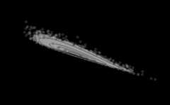


The figure shows how the transformations affect with shape of thedensity from which we simulate. In the bottom right plot the densitycontours suggests little dependence between the transformed components.The estimate of the probability of acceptance is approximately equal tothe 0.534 obtained for a 2-dimensional normal distribution withindependent components.
Finally, we show a plot of the sample and contours on the original\((\sigma, \xi\))-scale.
plot(x4, xlab="sigma", ylab="xi")
and an example of the output fromsummary.ru.
summary(x4)#> ru bounding box:#> box vals1 vals2 conv#> a 1.00000000 0.000000000 0.000000000 0#> b1minus -0.06636547 -0.107225819 0.006573398 0#> b2minus -0.06756121 -0.001105787 -0.107428499 0#> b1plus 0.07292561 0.123468775 0.005092513 0#> b2plus 0.06961246 -0.003093026 0.115104329 0#>#> estimated probability of acceptance:#> [1] 0.5319432#>#> sample summary#> sigma xi#> Min. :0.7156 Min. :-0.9428#> 1st Qu.:1.0228 1st Qu.:-0.6205#> Median :1.1088 Median :-0.5617#> Mean :1.1160 Mean :-0.5606#> 3rd Qu.:1.2004 3rd Qu.:-0.5023#> Max. :1.7745 Max. :-0.1537Example 2: log-normal density
If\(X\) has a log-normaldistribution with parameters\(\mu\)and\(\sigma\) then\(Z = \log X\) has a normal distribution withmean\(\mu\) and variance\(\sigma^2\). Therefore, we know that a logtransformation, i.e. a Box-Cox transformation with\(\lambda =0\), produces exact normality andwe find that the estimated probability of acceptance if greater when wetransform than when we don’t.
n<-10000# Sampling on original scale ----------------x1<-ru(logf=dlnorm, log=TRUE, d=1, n=n, lower=0, init=1)x1$pa#> [1] 0.5740858summary(x1)#> ru bounding box:#> box vals1 conv#> a 1.0000000 0.0000000 0#> b1minus -0.2023271 -0.2607045 0#> b1plus 1.5722199 8.0997951 0#>#> estimated probability of acceptance:#> [1] 0.5740858#>#> sample summary#> V1#> Min. : 0.01584#> 1st Qu.: 0.52102#> Median : 1.02848#> Mean : 1.64284#> 3rd Qu.: 1.95576#> Max. :30.91191# Box-Cox transform with lambda = 0 ----------------lambda<-0x2<-ru(logf=dlnorm, log=TRUE, d=1, n=n, init=0.1, trans="BC", lambda=lambda)x2$pa#> [1] 0.7944074To show how a user could implement their own transformation prior tosampling we use thetrans = "user" argument and supply theinverse Box-Cox transformation viaphi_to_theta and thelog-Jacobian vialog_j.
# Equivalently, we could use trans = "user" and supply the (inverse) Box-Cox# transformation and the log-Jacobian by handx3<-ru(logf=dlnorm, log=TRUE, d=1, n=n, init=0.1, trans="user", phi_to_theta=function(x)exp(x), log_j=function(x)-log(x))x3$pa#> [1] 0.7931472Sampling is performed using a normal density before transforming backto the log-normal scale.


We could also usefind_lambda_one_d to estimate asuitable value of\(\lambda\).
# Note: the default value of max_phi = 10 is OK here but this will not always be the case.lambda<-find_lambda_one_d(logf=dlnorm, log=TRUE)lambda#> $lambda#> [1] 0.06564725#>#> $gm#> [1] 0.9535484#>#> $init_psi#> [1] -0.06345259#>#> $sd_psi#> [1] 0.9753502We get a value of\(\lambda\) thatis close to zero and an estimated probability of acceptance that issimilar to before.
x4<-ru(logf=dlnorm, log=TRUE, d=1, n=n, trans="BC", lambda=lambda)x4$pa#> [1] 0.7914523Example 3: gamma density
The gamma distribution, with shape parameter\(\alpha\), provides a useful example becausewhen\(\alpha < 1\) the gammadensity is not bounded above. Therefore the ratio-of-uniforms cannot beused unless we use transformation to avoid this. Even if\(\alpha \geq 1\) we can improve theprobability of acceptance by transforming to approximate normality usinga cube root transformation(Wilson and Hilferty1931), i.e. a Box-Cox transformation with\(\lambda = 1/3\). We illustrate this for\(\alpha = 1\).
alpha<-1x1<-ru(logf=dgamma, shape=alpha, log=TRUE, d=1, n=n, lower=0, init=alpha)#> Warning in ru(logf = dgamma, shape = alpha, log = TRUE, d = 1, n = n, lower = 0, : The Hessian of the target log-density at its mode is not positive#> definite. This may not be a problem, but it may be that a mode#> at/near a parameter boundary has been found and/or that the target#> function is unbounded.#> It might be worth using the option trans = ``BC''.x1$pa#> [1] 0.6043757We get a warning because when\(\alpha =1\) the mode of a gamma distribution is at zero, the lower endpoint of the distribution. In this example it doesn’t matter because thedensity is finite at the mode and we are not relying on the mode beingat a turning point of the density. However, if we are using rotation ofaxes in a multidimensional example then we may have a problem becausethe rotation is based on an estimate of the Hessian of the density atthe mode.
Now we use a cube root transformation.
# Box-Cox transform with lambda = 1/3 works well for shape >= 1. -----------x2<-ru(logf=dgamma, shape=alpha, log=TRUE, d=1, n=n, trans="BC", lambda=1/3, init=alpha)x2$pa#> [1] 0.7937768Again we show howtrans = "user" can be used to useuser-defined transformation, this time supplying the value of\(\lambda\) usinguser_args.
# Equivalently, we could use trans = "user" and supply the (inverse) Box-Cox# transformation and the log-Jacobian by hand# Note: when phi_to_theta is undefined at x this function returns NAphi_to_theta<-function(x,lambda){ifelse(x*lambda+1>0,(x*lambda+1)^(1/lambda),NA)}log_j<-function(x,lambda)(lambda-1)*log(x)lambda<-1/3x3<-ru(logf=dgamma, shape=alpha, log=TRUE, d=1, n=n, trans="user", phi_to_theta=phi_to_theta, log_j=log_j, user_args=list(lambda=lambda), init=alpha)x3$pa#> [1] 0.7968762We could also usefind_lambda_one_d to set\(\lambda\): see the examples in thedocumentation forfind_lambda_one_d for details.
For\(\alpha < 1\) the gammadensity is very skewed and the density increases without limit at theorigin. A cube root transformation tends not to be sufficiently strongto produce a distribution for which the density is finite at its mode.We usefind_lambda_one_d to estimate a suitable value of\(\lambda\). We need to set a range ofvalues over which to evaluate the gamma density in order to estimate\(\lambda\). Here we cheat by using thegamma quantile function, something that wouldn’t usually beavailable.
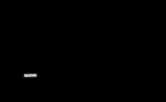
alpha<-0.1# Choose a sensible value of max_phimax_phi<-qgamma(0.999, shape=alpha)# [I appreciate that typically the quantile function won't be available.# In practice the value of lambda chosen is quite insensitive to the choice# of max_phi, provided that max_phi is not far too large or far too small.]max_phi<-qgamma(0.999, shape=alpha)lambda<-find_lambda_one_d(logf=dgamma, shape=alpha, log=TRUE, max_phi=max_phi)lambda#> $lambda#> [1] 0.06758891#>#> $gm#> [1] 0.008056577#>#> $init_psi#> [1] -0.0342618#>#> $sd_psi#> [1] 0.009372876x4<-ru(logf=dgamma, shape=alpha, log=TRUE, d=1, n=n, trans="BC", lambda=lambda)x4$pa#> [1] 0.7531822For a value of\(\alpha\) so closeto 0 the density is very peaked at the origin (see the plot on the leftbelow). After a transformation that is close to a log transformation thetarget density (see the plot on the right) is bounded above and theestimated probability of acceptance is similar to that of a normaldistribution.

Example 4: normal density
We show the effects of rotation of axes for the two- and three-dimensional normal density.
# two-dimensional normal with positive association ----------------rho<-0.9covmat<-matrix(c(1,rho,rho,1),2,2)log_dmvnorm<-function(x,mean=rep(0,d),sigma=diag(d)){x<-matrix(x, ncol=length(x))d<-ncol(x)-0.5*(x-mean)%*%solve(sigma)%*%t(x-mean)}# No rotation.x1<-ru(logf=log_dmvnorm, sigma=covmat, d=2, n=n, init=c(0,0), rotate=FALSE)# With rotation.x2<-ru(logf=log_dmvnorm, sigma=covmat, d=2, n=n, init=c(0,0))c(x1$pa,x2$pa)#> [1] 0.2353273 0.5368839The probability of acceptance is increased by the rotation of axes.These plots show why.


The three-dimensional case.
# three-dimensional normal with positive association ----------------covmat<-matrix(rho,3,3)+diag(1-rho,3)# No rotation. Slow !x3<-ru(logf=log_dmvnorm, sigma=covmat, d=3, n=n, init=c(0,0,0), rotate=FALSE)# With rotation.x4<-ru(logf=log_dmvnorm, sigma=covmat, d=3, n=n, init=c(0,0,0))c(x3$pa,x4$pa)#> [1] 0.05319488 0.31257814Again, pairwise plots of the simulated values illustrate the effectof the rotation of axes.
plot(x3, ru_scale=TRUE)
plot(x4, ru_scale=TRUE)