WO2010057078A2 - Method and system for generating spatially and temporally controllable concentration gradients - Google Patents
Method and system for generating spatially and temporally controllable concentration gradientsDownload PDFInfo
- Publication number
- WO2010057078A2 WO2010057078A2PCT/US2009/064555US2009064555WWO2010057078A2WO 2010057078 A2WO2010057078 A2WO 2010057078A2US 2009064555 WUS2009064555 WUS 2009064555WWO 2010057078 A2WO2010057078 A2WO 2010057078A2
- Authority
- WO
- WIPO (PCT)
- Prior art keywords
- gradient
- flow
- gradient material
- inlet port
- channel
- Prior art date
Links
Classifications
- G—PHYSICS
- G01—MEASURING; TESTING
- G01N—INVESTIGATING OR ANALYSING MATERIALS BY DETERMINING THEIR CHEMICAL OR PHYSICAL PROPERTIES
- G01N30/00—Investigating or analysing materials by separation into components using adsorption, absorption or similar phenomena or using ion-exchange, e.g. chromatography or field flow fractionation
- G01N30/02—Column chromatography
- G01N30/26—Conditioning of the fluid carrier; Flow patterns
- G01N30/28—Control of physical parameters of the fluid carrier
- G01N30/34—Control of physical parameters of the fluid carrier of fluid composition, e.g. gradient
- B—PERFORMING OPERATIONS; TRANSPORTING
- B01—PHYSICAL OR CHEMICAL PROCESSES OR APPARATUS IN GENERAL
- B01L—CHEMICAL OR PHYSICAL LABORATORY APPARATUS FOR GENERAL USE
- B01L3/00—Containers or dishes for laboratory use, e.g. laboratory glassware; Droppers
- B01L3/50—Containers for the purpose of retaining a material to be analysed, e.g. test tubes
- B01L3/502—Containers for the purpose of retaining a material to be analysed, e.g. test tubes with fluid transport, e.g. in multi-compartment structures
- B01L3/5027—Containers for the purpose of retaining a material to be analysed, e.g. test tubes with fluid transport, e.g. in multi-compartment structures by integrated microfluidic structures, i.e. dimensions of channels and chambers are such that surface tension forces are important, e.g. lab-on-a-chip
- B01L3/50273—Containers for the purpose of retaining a material to be analysed, e.g. test tubes with fluid transport, e.g. in multi-compartment structures by integrated microfluidic structures, i.e. dimensions of channels and chambers are such that surface tension forces are important, e.g. lab-on-a-chip characterised by the means or forces applied to move the fluids
- B—PERFORMING OPERATIONS; TRANSPORTING
- B01—PHYSICAL OR CHEMICAL PROCESSES OR APPARATUS IN GENERAL
- B01L—CHEMICAL OR PHYSICAL LABORATORY APPARATUS FOR GENERAL USE
- B01L3/00—Containers or dishes for laboratory use, e.g. laboratory glassware; Droppers
- B01L3/50—Containers for the purpose of retaining a material to be analysed, e.g. test tubes
- B01L3/502—Containers for the purpose of retaining a material to be analysed, e.g. test tubes with fluid transport, e.g. in multi-compartment structures
- B01L3/5027—Containers for the purpose of retaining a material to be analysed, e.g. test tubes with fluid transport, e.g. in multi-compartment structures by integrated microfluidic structures, i.e. dimensions of channels and chambers are such that surface tension forces are important, e.g. lab-on-a-chip
- B01L3/502769—Containers for the purpose of retaining a material to be analysed, e.g. test tubes with fluid transport, e.g. in multi-compartment structures by integrated microfluidic structures, i.e. dimensions of channels and chambers are such that surface tension forces are important, e.g. lab-on-a-chip characterised by multiphase flow arrangements
- B01L3/502776—Containers for the purpose of retaining a material to be analysed, e.g. test tubes with fluid transport, e.g. in multi-compartment structures by integrated microfluidic structures, i.e. dimensions of channels and chambers are such that surface tension forces are important, e.g. lab-on-a-chip characterised by multiphase flow arrangements specially adapted for focusing or laminating flows
- B—PERFORMING OPERATIONS; TRANSPORTING
- B01—PHYSICAL OR CHEMICAL PROCESSES OR APPARATUS IN GENERAL
- B01L—CHEMICAL OR PHYSICAL LABORATORY APPARATUS FOR GENERAL USE
- B01L2300/00—Additional constructional details
- B01L2300/08—Geometry, shape and general structure
- B01L2300/0809—Geometry, shape and general structure rectangular shaped
- B01L2300/0816—Cards, e.g. flat sample carriers usually with flow in two horizontal directions
- G—PHYSICS
- G01—MEASURING; TESTING
- G01N—INVESTIGATING OR ANALYSING MATERIALS BY DETERMINING THEIR CHEMICAL OR PHYSICAL PROPERTIES
- G01N1/00—Sampling; Preparing specimens for investigation
- G01N1/28—Preparing specimens for investigation including physical details of (bio-)chemical methods covered elsewhere, e.g. G01N33/50, C12Q
- G01N1/40—Concentrating samples
- G01N1/405—Concentrating samples by adsorption or absorption
- G—PHYSICS
- G01—MEASURING; TESTING
- G01N—INVESTIGATING OR ANALYSING MATERIALS BY DETERMINING THEIR CHEMICAL OR PHYSICAL PROPERTIES
- G01N1/00—Sampling; Preparing specimens for investigation
- G01N1/28—Preparing specimens for investigation including physical details of (bio-)chemical methods covered elsewhere, e.g. G01N33/50, C12Q
- G01N1/40—Concentrating samples
- G01N1/4077—Concentrating samples by other techniques involving separation of suspended solids
- G01N2001/4088—Concentrating samples by other techniques involving separation of suspended solids filtration
- G—PHYSICS
- G01—MEASURING; TESTING
- G01N—INVESTIGATING OR ANALYSING MATERIALS BY DETERMINING THEIR CHEMICAL OR PHYSICAL PROPERTIES
- G01N30/00—Investigating or analysing materials by separation into components using adsorption, absorption or similar phenomena or using ion-exchange, e.g. chromatography or field flow fractionation
- G01N30/02—Column chromatography
- G01N30/26—Conditioning of the fluid carrier; Flow patterns
- G01N30/28—Control of physical parameters of the fluid carrier
- G01N30/34—Control of physical parameters of the fluid carrier of fluid composition, e.g. gradient
- G01N2030/342—Control of physical parameters of the fluid carrier of fluid composition, e.g. gradient fluid composition fixed during analysis
- Y—GENERAL TAGGING OF NEW TECHNOLOGICAL DEVELOPMENTS; GENERAL TAGGING OF CROSS-SECTIONAL TECHNOLOGIES SPANNING OVER SEVERAL SECTIONS OF THE IPC; TECHNICAL SUBJECTS COVERED BY FORMER USPC CROSS-REFERENCE ART COLLECTIONS [XRACs] AND DIGESTS
- Y10—TECHNICAL SUBJECTS COVERED BY FORMER USPC
- Y10T—TECHNICAL SUBJECTS COVERED BY FORMER US CLASSIFICATION
- Y10T436/00—Chemistry: analytical and immunological testing
- Y10T436/25—Chemistry: analytical and immunological testing including sample preparation
- Y10T436/2575—Volumetric liquid transfer
Definitions
- the present inventionis directed to methods and systems for rapidly generating concentration gradients of diffusible molecules, polymers, beads and cells. Further, the invention is directed to methods and systems for rapidly generating spatially and temporally controllable concentration gradients of these gradient materials in a portable microfluidic device.
- Natural materialsexhibit anisotropy with variations in soluble factors, cell distribution, and matrix properties. The ability to recreate the heterogeneity of the natural materials is a major challenge for investigating cell-material interactions and for developing biomimetic materials.
- Anisotropic materialsare highly important for many natural and engineered systems.
- anisotropic materials in natureinclude marbles, tree trunks and squid beaks.
- engineered anisotropic materialsinclude the birefringent crystals of prisms, the metal wood head of golf clubs and the aluminum alloys used in aircraft and rockets. Spatial anisotropy in materials is especially prominent in cellular microenvironments in vivo where heterogeneous distributions of cells and molecules exist within spatially varying extracellular matrices (ECM). Molecular concentration gradients play an important role in biological phenomena such as chemotaxis, morphogenesis and wound healing. Meanwhile, the graded variations of ECM and cell concentration at the tissue interface (e.g. bone-cartilage interface, dentino- enamel junctions) are nature' s solution for connecting mechanically mismatched tissues. Creating chemical and material gradients to mimic the heterogeneity of cellular environments is important for investigating cell-matrix interaction and for developing biomimetic materials for tissue engineering.
- ECMextracellular matrices
- the first methodis advantageous for producing stable complex gradients, but the experiments are not compatible with non-adherent and weakly adherent cells and the shear/drag force generated by the flow may alter the intercellular signaling pathways.
- pumping systems with external connectionsi.e. tubing and valves
- external connectionsi.e. tubing and valves
- the second approachnormally requires larger gradient generation times and the gradient produced is unstable and hard to maintain over long time periods. Gradients have also been formed parallel to the direction of flow. Goulpeau et al. built up longitudinal concentration gradients along their microchannel by using transient dispersion along the flow. Kang et al. developed a device that generated concentration gradients parallel to the direction of flow by using a convective-diffusive balance in a counter -flow configuration. Although these approaches could be used to rapidly generate concentration gradients in less than one minute, they still required external components i.e. hydrostatic pumps or valves to introduce and control the flows within the channels.
- the surface tension difference between the larger drop of solution at the outlet and smaller drop of solution at the inletwas used to pump the small drop of liquid through the micro-channel, which has been shown to be a powerful high-throughput microfluidic tool for cell culturing. Evaporation has also been used as driving force in pump- less' microfluidic devices. Evaporation is a well-known issue when handling small liquid volumes, especially in microfluidic devices. While the loss of volume due to evaporation may cause unwanted effects such as the change of concentrations or osmolality of the fluid solution; evaporation in microfluidic devices has proven to be a useful tool in several applications, including generating slow, steady flows in microchannels used for chromatography, DNA analysis devices, and sample concentration.
- the present inventionis directed methods and systems for rapidly generating concentration gradients of diffusible materials (including chemical compounds and biologic molecules), polymers, beads, particles and cells in the channel of a microfluidic device.
- diffusible materialsincluding chemical compounds and biologic molecules
- alternating flowsare induced in the channel to produce multi- centimeter long concentration gradients.
- Methods and systems according to the inventionuse alternating flows and hydrodynamic stretching to rapidly generate long gradients of these gradient materials and long cross- gradients of two species of gradient materials in a simple microchannel.
- the length of the concentration gradientcan be predetermined for wide range of material properties.
- a poly( ethylene-glycol) hydrogel gradient, a porous collagen gradient and a composite material with a hyaluronic acid/gelatin cross- gradientcan be generated with continuous variations in material properties and in their ability to regulate cellular response.
- the present inventioncan be useful for creating anisotropic biomimetic materials and high-throughput platforms for investigating cell-mi croenvironment interaction.
- methods and systems according to this embodimentutilize a forward flow induced by the passive-pumping and a reversed flow induced by evaporation to rapidly establish centimeter-length concentration gradients of molecules along the channel of a simple and portable microfluidic device.
- Passive-pumpingis used to generate a forward flow from the inlet to the outlet of the channel, which introduced the gradient material (molecules of interest) into the microfluidic device in a rapid and simple manner and initiated a concentration gradient profile of the molecules due to the parabolic shape of the front flow.
- An evaporation-induced backward flow from the outlet to the inlet of the channelfollowed the forward flow resulting in the formation of dynamic concentration gradients of the molecule.
- methods and systems according to this embodimentutilize a pumping mechanism that produce fast alternating flows, which continually lengthen the gradient.
- the methods and systems according to this embodimentutilize the pumping mechanism to produce fast alternating flows of a second gradient material to generate a cross gradient.
- a non- viscous solutionsuch as a buffered solution is input into the channel of the microfluidic device and the gradient material is pumped into in one or more cycles of alternating forward and backward flows.
- Each cyclecan be defined to include injecting into the inlet a predefined volume of gradient material at a predefined flow rate, imparting a predefined forward flow velocity on the gradient material, waiting a predefined period of time to allow for diffusion and withdrawing a predefined volume of gradient material from the inlet at a predefined flow rate, imparting a predefined backward flow velocity on the gradient material.
- a predefined waiting period to allow for diffusion between cyclescan be provided.
- the length of the gradient in the channelcan determined as function of the flow velocity and the amount of time that the gradient material flows.
- the present inventionprovides methods and systems for simple and rapid generation of relatively long concentration gradients in portable microfluidic devices.
- the present inventioncan provide that : 1) the concentration gradient is generated by dispersion, the combined effect of convection and molecular diffusion, and flow reversal, which changes the direction of the parabolic flow; 2) due to the convection-driven nature, the process of gradient generation was rapid (within several minutes), highly dynamic (throughout the backward flow stage) and spatially/temporally controllable (by controlling the evaporation-induced backf low); 3) the gradient can be formed by consuming low amounts of the gradient material (particles, cells, or molecules, etc.) of interest; 4) centimeter-length concentration gradients can be generated parallel to the flow direction along the channel; and 5) the process is simple and highly reproducible in a portable microfluidic device, requiring only a pipette for implementation.
- the present inventionis directed to a versatile platform for generating centimeter scale gradients of a broad range of gradient materials, from molecular to micron scale, in seconds to minutes.
- Particle and cell concentration gradientscan be produced by high-speed alternating fluidic shear in a simple microfluidic channel.
- flow sequences according to the inventioncan be used to generate long and laterally uniform gradients, including 2-3 cm gradients of fluorescent dyes.
- the same flow sequencescan also be used to create gradients of hydrogels and cross gradients composite materials (such as, HA- gelatin, which possessed a gradient in cell- attachment).
- gradient generationcan be controlled using a formula for estimating gradient growth which is useful over a wide range of P ⁇ clet numbers and channel geometries. [017] It is an object of the invention to generate a concentration gradient of a gradient material over a predefined length of a microfluidic channel. [018] It is another object of the invention to rapidly generate a concentration gradient of a gradient material over a predefined length of a microfluidic channel.
- FIG. 1is a diagrammatic view of a microfluidic device according to the invention.
- FIG. 2is a flow chart of a process for generating concentration gradients according to the invention.
- FIGS. 3A-3Dshow a diagrammatic view of a process for generating concentration gradients according to the invention.
- FIGS. 4A-4Dshow experimental and simulated results of dynamic gradient generation according to the invention.
- FIGS. 5A-5Bshow diagrammatic views of gradient generation by dispersion according to the invention.
- FIG. 6Ashows diagrammatic views of the evolution of the concentration gradient over time due to molecular diffusion, according to the invention.
- FIG. 6Bshows simulated results of the evolution of the concentration gradient over time due to molecular diffusion, according to the invention.
- FIG. 7is a diagrammatic view of a microfluidic device according to the invention.
- FIG. 8is a flow chart of a process for generating concentration gradients according to the invention.
- FIG. 9is a flow chart of a process for generating a cross-gradient according to the invention.
- FIGS. 10A- 1ODshow diagrammatic views of modes of gradient generation in channel flow according to the invention.
- FIGS. 1 IA-11Cshow diagrammatic views of the generation of long range molecular gradients according to the invention.
- FIGS. 12A-12Eshow diagrammatic views of the generation of long range particle, cellular and material gradients according to the invention.
- FIGS. 13A-13Dshow diagrammatic ⁇ ew of a cross gradient generated according to the invention.
- the present inventionis directed methods and systems for rapidly generating concentration gradients and cross-gradients of gradient materials (e.g., diffusible molecules, chemical compounds, biologic molecules, polymers, beads, particles, and cells) in the channel of a microfluidic device.
- gradient materialse.g., diffusible molecules, chemical compounds, biologic molecules, polymers, beads, particles, and cells
- alternating flowsare introduced in the channel of the microfluidic device to produce multi-centimeter long concentration gradients.
- Methods and systems according to one embodiment of the inventionutilize a forward flow induced by the passive-pumping and a reversed flow induced by evaporation to rapidly establish centimeter-length concentration gradients of molecules along the channel of a simple and portable microfluidic device.
- Passive-pumpingis used to generate a forward flow from the inlet to the outlet of the channel, which introduced the molecules of interest (with volume less than lO ⁇ L) into the microfluidic device in a rapid and simple manner and initiated a concentration gradient profile of the molecules due to the parabolic shape of the front flow.
- Passive-pumpingincludes applying one or more droplets to the inlet port of the microfluidic channel.
- one methodology used to generate the concentration gradientrelies on the flow properties and the combined effect of convection and diffusion of the gradient materials into the base solution in the microfluidic channel.
- the flowis essentially fully-developed laminar Poiseuille flow in a rectangular channel, a textbook example where the Navier-Stokes equations admit an exact solution.
- the Peclet numbers for the forward and backward flowsare approximately 1000 and 10, respectively.
- the chemical transportis mainly due to convection; since the flow is essentially axial, the transport in the transverse direction is mainly due to molecular diffusion. This type of chemical spreading, involving both axial convection and transverse molecular diffusion, is called Taylor dispersion.
- the stabilized concentration gradient of a cardiac toxinwas used to test the toxicity response of HL-I cardiac cells seeded within the channel.
- the present inventionprovides for ease of use, portability, low consumption and scalability and can be useful for various biological and chemical processes where rapid generation of long- range concentration gradients can be used.
- the microfluidic devicecan be fabricated by using standard soft-lithography methods. Photomasks with channel patterns were designed using AutoCAD and printed on transparencies with 20,000 dpi resolution (CAD/Art Services, Inc., Bandon, OR). Master molds patterned with lOO ⁇ m thick resist were made by patterning a negative photoresist (SU- 8 2050, Microchem, MA) on a silicon wafer. PDMS molds were fabricated by curing prepolymer (Sylgard 184, Essex Chemical, Midland, MI) on silicon masters patterned with S U- 8 photoresist. Briefly, PDMS molds were generated by mixing silicone elastomer and curing agent (10:1 ratio).
- the PDMS prepolymerwas poured on the silicon master that was patterned with photoresist and cured at 70 ° C for 2h. PDMS molds were then peeled off from the silicon wafer. The inlet and outlet of the microchannel were created by a sharp punch (hole radius: 0.4 mm) for medium perfusion and cell seeding.
- the microfluidic deviceconsisted of a top PDMS fluidic channel and a bottom glass slide.
- the top fluidic channelwas lOO ⁇ m (height) x 50mm (length) x 1.6mm (width), which was bonded to the bottom glass slide after treatment by oxygen plasma (Harrick Scientific, Pleasantville, NY). [043] Fig.
- the microfluidic device 100includes a top portion 110 into which the microfluidic channel 116 is formed.
- the top portion 110can be bonded to a bottom portion 120.
- the microfluidic device 100also includes an inlet port 112 connected to one end of the microfluidic channel 116 and an outlet port 114 connected to the other end of the microfluidic channel 116.
- the channelcan be filled with a buffered solution (or culture medium) and a large drop 134 of the buffered solution can be placed on the outlet port 114.
- Figs. 2shows a flow chart of the process of generating the concentration gradient in the microfluidic channel 116 according to one embodiment of the invention.
- Figs. 3A- 3Dshow a diagrammatic representation of process of generating the concentration gradient in the microfluidic channel 116 according to one embodiment of the invention.
- the microfluidic channel 116having an inlet port 112 and an outlet port 114, in which the concentration gradient is to be created, is provided at 202.
- the microfluidic channel 116can be part of a microfluidic device 100 such as shown in Fig. 1.
- the microfluidic channel 116is prefilled with a non -viscous solution, such as a buffer solution or culture medium, at 204.
- a non -viscous solutionsuch as a buffer solution or culture medium
- a large drop 134 of the non -viscous solutionis placed on the outlet port 114 and one or more small drops 132 are placed on the inlet port 112 to initiate the passive-pumping process and causing the gradient material to flow forward in the channel 116, from the inlet port to the outlet port as shown in Fig. 3B.
- the gradient material at the inlet portwas allowed to evaporate to cause the gradient material to flow backward, from the outlet port to the inlet port at 208 and as shown in Fig. 3C.
- the desired length of the concentration gradientis generated and the inlet port 112 and the outlet port 114 are sealed to stabilize the gradient at 210 and as shown in Fig. 3D.
- the size of the large drop 134can determined as a function of the desired passive- pumping action to induce the desired flow, given the materials used.
- the large drop 134can range from 100 ⁇ L to 500 ⁇ L.
- the small drop 132can be determined as a function of the desired flow.
- the small dropcan be a small droplet and can range from 1 ⁇ L to 5 ⁇ L.
- Evaporation at the inlet portcan be naturally induced, such as the result of ambient environmental conditions or can be actively induced by subjecting the environment adjacent to the inlet port to decreasing pressure or increasing temperature.
- the length of time that the evaporation-driven backflow is allowed to continuecan be determined by the desired length of the concentration gradient.
- the time ranged from 10 minutes to 50 minutes and the time of the backflowcan be longer than 50 minutes depending on the characteristics of the system and the desired length of the concentration gradient.
- the microfluidic devicecan be cooled, frozen, freeze- dried, exposed to UV energy or otherwise processed further to cause the solution in which the gradient was generated to solidify allowing the top portion of the microfluidic device to be removed so that the concentration gradient can be exposed and/or harvested.
- Figs. 4A-4Dshow the experimental and simulation results of dynamic gradient generation in the microfluidic channel.
- Fig. 4Ashows fluorescence images of the forward flow of a solution containing FITC-Dextran into the microfluidic channels produced by passive-pumping. The corresponding simulation results obtained by the finite element method are positioned directly below each experimental fluorescence images. The vertical color scale denotes fluorescence intensity.
- Fig. 4Bshows fluorescence images of the generation of a dynamic gradient of FITC-Dextran produced by evaporation-driven backward flow. The corresponding simulation results obtained by finite element method are positioned below the experimental images.
- Fig. 4Cshows experimental results and Fig.
- FIG. 4Dshows simulation results of the normalized fluorescence signal of FITC-Dextran along the channel at different times during the backward flow.
- Figs. 5A-5Bshow the gradient generation by dispersion (convection and diffusion).
- Fig. 5Ashows the effect of flow reversal on concentration gradient.
- Fig. 5Bshows the simulated results that verify the effects of dispersion on the formation and dynamic change of the concentration gradient, including top-down and cross-sectional views of the simulation results of the concentration profiles.
- Fig. 5Bishows the concentration profile at the end of the forward flow.
- Fig. 5Biishows the concentration profile after 8min of backward flow.
- Fig. 5Biiishows the concentration profile after 16min of backward flow.
- Fig. 5Bivshows the concentration profile after 32min of backward flow.
- Figs. 6A-6Dshow the evolution of the concentration gradient profile due to molecular diffusion after backward flow was stopped.
- Fig. 6 Ashows FITC-D extran in the microfluidic channel for 4h with flow stopped by oil sealing (top) and for 12h with flow stopped by maintaining a 100% humidity environment (bottom).
- Fig. 6B and 6Cshow the simulation results of the dynamic concentration gradient driven by molecular diffusion over one day.
- Fig. 6Bshows the result for molecules with diffusivity of 10 " cm s " and
- Fig. 6Cshows the results for molecules with diffusivity of 10 "6 Cm 2 S "1 .
- the channelwas initially filled with Dulbecco's Phosphate Buffered Saline (DPBS, Gibco, Carlsbad, CA).
- DPBSDulbecco's Phosphate Buffered Saline
- a 200 ⁇ L drop of DPBSwas pipetted onto the outlet opening and a 2 ⁇ L drop of DPBS containing the molecule of interest was dropped onto the inlet opening and subsequently entered the channel automatically.
- a second drop containing 2 ⁇ Lwas pipetted onto the inlet to continue the forward flow.
- the inletwas not refilled, the forward flow would stop and a backflow occurred due to evaporation at the room humidity ( ⁇ 65%).
- fluorescein isothiocyanate-dextran(FITC-D extran, molecular weight (MW): 1OkD) was used as the model molecule, and the fluorescence image series was captured using a Kodak Gel Logic 100 Imaging System, shown in Figs. 4-6. The average fluorescence intensity along the whole channel was quantified by ImageJ software.
- the evaporation-driven flowwas stopped by either sealing the inlet port and optionally, the outlet port with a drop of mineral oil or putting the microfluidic device into an enclosure with 100% humidity.
- V - UQ (2 )
- Table 1 in Appendix Asummarizes the input parameters used for the numerical simulations.
- the channel geometrywas set as 5cm x 1600 ⁇ m x lOO ⁇ m and FTTC- Dextran was used as the model dye molecules.
- concentrationswere extracted from the centerline along the channel and normalized with the maximum concentration at the inlet of the channel.
- HL-I cellsCardiac muscle cell line
- FBSFetal Bovine Serum
- Penicillin / Streptomycin1% Norepinephrine
- L-Glutamine1% L-Glutamine at 37 oC in a humidified 5% CO2 / 95% air incubator.
- the bottom glass slidewas coated with a mixture of extracellular matrix (0.02% gelatin (w/w) and 5 ⁇ g/mL fibronectin) after the top channel was bonded to the bottom glass slide.
- the cellswere trypsinized and seeded through the outlet port using dynamic seeding at a cell density of 2 x 10⁶ cells ⁇ iL-1 that allowed uniform cell distribution. Cells were cultured for 2 h to ensure attachment. The medium was then changed and 3 drops of 2 ⁇ L medium containing 2OmM Alpha- cypermethrin were introduced by passive pumping and a concentration gradient was established by leaving the microfluidic device in the hood for 5min to allow for evaporation- induced backflow. The microfluidic device was then transferred to a humidified incubator where the concentration gradient of the toxin was stabilized and the cells were treated for 4h.
- Cell morphology and viabilitywas characterized by peeling off the top channel and incubating the cells with live/dead dyes (2 ⁇ L CaIc ein AM and 0.5 ⁇ L Ethidium homodimer-1, Molecular Probes, California) in ImL DPBS for lOmin. ImageJ was used to quantify the fluorescence images of live-dead staining of the cells. At least three images were used for quantification of the cell viability.
- a stable concentration gradientwas produced using the process shown in Fig. 3.
- Fig. 3shows a schematic diagram of the gradient generation and stabilization process: A) Microfluidic channel was first filled with DPBS; a large drop of DPBS was placed on the outlet opening and a small drop of the gradient material containing diffusible molecules was pipetted on the inlet opening, B) solution was introduced into the channel automatically by the passive-pump-induced forward-flow; C) a concentration gradient of molecules was generated during the evaporation-based backward flow; D) the gradient profile could be stabilized by stopping the evaporation, either by sealing the inlet with mineral oil or by maintaining the microfluidic device at 100% humidity.
- the microfluidic channelwas initially filled with DPBS, and a 200 ⁇ L drop of DPBS was pipetted onto the outlet.
- a small drop of 2 ⁇ L DPBS containing FITC- Dextranwas then dropped onto the inlet (Fig. 3A) and entered the channel automatically due to the differential surface tensions between the drops (Fig. 3B).
- a second dropwas pipetted onto the inlet to continue the forward flow.
- three dropswere sufficient for the fluid to reach the desired distance in the channel, in this example, the outlet end of the 5cm-long channel.
- the forward flow ratewas ⁇ lmm/s as measured experimentally and calculated analytically.
- a centimeter long concentration gradient with uniform cross- sectional distributionis formed after 16min of backward flow for molecule with a diffusivity of 1.7x10⁻⁶ cm2/s (i.e. FITC-Dextran) as shown in Fig. 5B iii.
- the concentrationforms a slightly inverted parabolic profile.
- the uniformity of the concentration distributionwas not significantly affected, and a relatively uniform concentration gradient moved backward toward the inlet as shown in Fig. 5B iv.
- the timescale for molecular diffusion across a distance Lis L /(xD), where D is the molecular diffusivity.
- the timescales for vertical and horizontal mixing of FITC-Dextran across the lOO ⁇ m height and 1.6mm width of the channelare therefore 6 seconds and 25 minutes, respectively.
- the chemical concentrationis essentially uniform vertically across the microchannel, and it suffices to consider only its horizontal variation, as we have done.
- the timescale for molecular diffusion across the width of the channelis significantly greater than the duration of the forward flow and commensurate with the timescale of the backward flow. It is therefore instructive to consider the role of the backward flow on gradient generation.
- a particular concentration gradientwas stabilized using two methods to stop the flow. As shown in Fig. 3D and Fig. 6 A, evaporation from the inlet can be prevented either by sealing with mineral oil or by placing the microfluidic device in an environment with 100% humidity (water bath or cell incubator).
- the oil sealing approachcould stabilize a particular concentration gradient profile for up to 4h before evaporation through the PDMS layer became noticeable (indicated by the small cavities in the fluorescence image in Fig. 6A, while a concentration gradient profile could be stabilized under 100% humidity for at least 12h.
- Centimeter-long concentration gradients of chemicals with molecular diffusivities of 10 "7 cm 2 /s and 10 "6 cm 2 /sremain within 10% of their initial states over time intervals of approximately 28h and 2.8h, respectively.
- Example 3Stabilized concentration gradient for cytotoxicity testing.
- a cardiac muscle cell line(HL-I) is used to investigate the cytotoxicity of Alpha-cypermethrin, a cardiac toxin.
- Three drops of 2 ⁇ L medium containing 2OmM Alpha-cypermethrinwere loaded consecutively into the micro-devices with HL-I cells seeded along the channel.
- a concentration gradient of the toxinwas established by evaporation when the micro device was left at ambient conditions for 5min (5min exposure does not cause severe damage to cell viability) and the gradient was stabilized when the micro device was transferred to the humidified incubator.
- HL-I cells exposed to the toxin concentration gradient for 4hexhibited distinguishable morphologies along the channel, with more severe effects observed in the regions containing higher concentrations of toxin.
- the drastic morphological change of HL-I cells exposed to various concentrations of toxinwas also observed when the cytotoxicity testing was conducted with HL-I cells seeded in a 96-well plate.
- the cytotoxicity of the toxin gradientwas further tested on the HL-I cells by conducting a live-dead assay. A correlation of cell viability was found with the toxin concentration gradient along the channel.
- the experimental conditions used in this exampleestablished a concentration gradient of the toxin from 12.5mM to OmM along the 5cm-length channel based on the assay conducted in this example.
- the gradient generation processis highly reproducible at ambient conditions (i.e. 22 C, 30% relative humidity). Variations in temperature and humidity in the laboratory mainly affect the gradient generation process by slightly altering the backward flow rate induced by evaporation; their effects on the forward flow and the diffusion of the molecular are generally considered negligible.
- the flowis essentially fully developed Poiseuille flow throughout the rectangular channel. Regions of adjustment to the fully developed flow exist at the ends of the channel. However, based on the Reynolds numbers (0.1 and 0.001) of the forward and backward flows, the extent of these adjustment regions is short: approximately the channel height. Thus, throughout the channel the flow is essentially fully-developed Poiseuille flow.
- the concentration gradient profile according to the present inventioncan be easily altered and controlled by choosing the initial analyte concentration in the applied drops and by manipulating the timing of the forward and backward flow. The factors affecting the flow properties, such as the fluid viscosity, the pressure difference between the inlet and outlet, the rate of evaporation and the geometry of the microfluidic channel affect the gradient generation.
- Methods and systems according to an alternative embodiment of the inventionutilize a pumping device, such a syringe pump, to drive fast alternating flows which continually lengthen the concentration gradient in the channel.
- a pumping devicesuch as a syringe pump
- This embodiment of the inventionprovides for rapidly generating multi- centimeter long concentration gradients along the channel in a simple and portable microfluidic device.
- Active pumpingis provided to drive forward and backward flows in the channel.
- active pumpingcan be used to rapidly generate long cross gradients of two gradient materials in the channel of a simple and portable microfluidic device.
- Fig. 7shows a diagram of a microfluidic device 700 according to an embodiment of the invention.
- the microfluidic device 700includes a top portion 710 into which the microfluidic channel 716 is formed.
- the top portion 710can be bonded to a bottom portion 720.
- the microfluidic device 700also includes an inlet port 712 connected to one end of the microfluidic channel 716 and an outlet port 714 connected to the other end of the microfluidic channel 716.
- the inlet port 712is connected by tubing to a pump 740, such as a syringe pump, which can inject and withdraw a predefined amount of the gradient material solution to the inlet port 712.
- a pump 740such as a syringe pump
- the channelcan be filled with a buffered solution and optionally, a large drop 734 of the buffered solution can be placed on the outlet port 714.
- the pump 740is operated or programmed to inject a predefined volume of the gradient material solution at a predefined flow rate into the inlet port 712, to induce a forward flow rate in the channel for a predefined time.
- the pump 740is stopped for a predefined period of time to allow the diffusion to mix the solution vertically.
- the pump 740is operated or programmed to withdraw a predefined volume of the gradient material solution at a predefined flow rate from the inlet port 712 to stretch the concentration gradient.
- the cyclecomprising a forward flow, a delay and a backward flow can be repeated (with an optional delay in between) until the concentration gradient grows to fill the channel.
- an optional forward flowcan be induced in the channel to increase the length of the gradient.
- the inlet port and optionally, the outlet portcan be sealed to stop the growth and stabilize the concentration gradient.
- Figs. 8shows a flow chart of the process of generating the concentration gradient in the microfluidic channel 716 according to an alternative embodiment of the invention.
- the microfluidic channel 716having an inlet port 712 and an outlet port 714, in which the concentration gradient is to be created, is provided at 802.
- the microfluidic channel 716can be part of a microfluidic device 700 such as shown in Fig. 7.
- the microfluidic channel 716is prefilled with a non-viscous solution, such as a buffer solution or culture medium, at 804.
- a large drop 734 of the non -viscous solutionis optionally placed on the outlet port 714 and the pump 740 is operated or its program initiated to inject a predefined volume of gradient material solution into the inlet port 712 to cause a forward flow of the gradient material in the channel 716, from the inlet port to the outlet port.
- the pump 740is stopped for a predetermined delay period to allow for diffusion, at 808.
- the pump 740is reversed (either manually operated or as part of a program) to withdraw a predetermined amount of gradient material solution at a predetermined flow rate, to cause a backward flow of the gradient material in the channel toward the inlet port 712, at 810.
- cycle of forward flow, delay and backward flowcan be repeated using the same or different flow parameters (volume, flow rate and time delay) at 812 to grow the concentration gradient to the desired length.
- an optional delayfor example, 814) and, at 816, an optional forward flow can be caused by pumping a predetermined amount of gradient solution into the channel 716 to further stretch the concentration gradient.
- the inlet port and, optionally, the outlet portcan be sealed (such as with oil or 100% humidity), at 818 to stabilize the concentration gradient in the channel 716.
- Fig. 10shows a schematic for gradient generation and modes of spreading in channel flow.
- Fig. 1OAshows particles spreading due to hydrodynamic stretching.
- Fig. 1OBshows how diffusion suppresses longitudinal spreading.
- Fig. 1OCshows the effect of gravity on gradient material.
- Fig. 1ODshows advection and diffusion of solute dissolved in the flow, for high P ⁇ clet number (high flow rate or small diffusivity) and low P ⁇ clet number (low flow rate or high diffusivity).
- fluidic shear-driven stretchingis the primary mode of gradient generation.
- a particle in the center of the channelmoves faster than one at the wall and the two spread apart at a rate proportional to the maximum channel velocity.
- a gradientforms in the laterally averaged concentration profile.
- Diffusionacts to suppress hydrodynamic stretching by reducing the mean variation in particle speeds slowly moving particles near the wall diffuse toward the centre and accelerate, while fast moving particles near the center diffuse toward the wall and decelerate as shown in Fig. 1OB.
- diffusionis negligible.
- high-speed (mm/s) flow shear-driven stretchingcan be used to generate gradients of a wide range of gradient materials (e.g. molecules, cells and microbeads) along a simple microchannel.
- the transported specieswas introduced into one end of the channel and the flow began.
- the concentration profilewas hydrodynamically stretched and the initially short, steep gradient in concentration spread (Appendix B, Fig ICi).
- the profile stretchingwas suppressed by lateral molecular diffusion, so that larger spreading was observed for larger P ⁇ clet numbers.
- the flowwas stopped before the gradient reached the end of the channel.
- the flowwas then reversed and stopped before the gradient reached the opposite end of the channel (Appendix B, Fig. ICiii).
- the cyclewas repeated until a gradient of sufficient length was obtained. As the gradient grew and filled the channel, the flow segments became shorter. These short duration flows laterally smoothed the concentration profile by shortening the spatial lags between the wall and centreline concentration profiles.
- H 2 ZDis seconds to minutes and W 2 ZD is hours to days. Since the concentration gradients are generated in seconds to minutes, their evolution falls in the early to intermediate dispersion regime. Approximate theoretical descriptions valid for early, intermediate, and late times exist for many geometries, including rectangular channels, cylindrical tubes, and channels with smooth cross-sections. In these approximate theories, the cross-section ally averaged concentration has the classic erfc profile (Appendix B, IL3c) with a dispersivity D , which plays the role of an effective diffusivity, though orders of magnitude larger than the molecular diffusivity.
- the theories listed abovegive different forms for the dispersivity depending on the time regime and the geometry. All theories listed are for uni-directional flow; the effects of flow reversal can be computed numerically.
- a finite element code(Comsol AB) can be determined to solve the advection-diffusion equation in the microchannel on a rectangular grid (Supp. Fig. 2).
- Flow reversalis modelled by initializing the computational model with the concentration profile following the previous flow segment or pure diffusion segment and running the steady flow backwards.
- the resulting numerically computed concentration profileswere cross-sectionally averaged and the gradient length ⁇ was extracted.
- the gradient length ⁇is defined as the distance between 10% and 90% of the maximum concentration, which captures the most linear, and therefore usable, portion of the concentration profile.
- Fig. 11shows the generation of long-range molecular gradients.
- FIG. 1 IBshows long range molecular gradient generation in backward flow: top-down view of fluorescent FITC- Dextran gradient and quantification of centerline (C), wall (W), cross-sectionally averaged (A) gradient profiles, gradient length ⁇ and spatial lag ⁇ .
- Fig. 11 Cshows long range molecular gradient generation in alternating flow cycles: top-down view of fluorescent FITC- Dextran gradient and quantification along centerline, including gradient length ⁇ and spatial lag ⁇ .
- Fig. 12shows the generation of long-range gradient of particles, cells and materials.
- Fig. 12Ashows an SEM image (with low and high magnification) of PEG-DA hydro gel gradient.
- Figs. 12B and Cshow an image of fluorescent particles (diameter 5 ⁇ m) and endothelial cells, respectively.
- Fig. 12Dshows the quantification of the continuous variance in thickness of the hydrogel gradient.
- FIG. 12Eshows the quantification of the relative density profiles of endothelial cells and fluorescent particles (with diameters of 5, 10 ⁇ m).
- the thickness of the dried hydrogel gradientgradually increased from ⁇ 10 ⁇ m in the region formed with 5wt% PEG-DA to ⁇ 40 ⁇ m in the region with 40wt% PEG-DA.
- thermally cross-linked collagen gradientswere produced and visualized after free-drying.
- the porous 3D collagen meshexhibited continuous changes of fibril density (Fig. 12B).
- the gradient platform according to the present inventioncan also be used to produce material gradients of various mi crop articles. Using high flow speeds (mm/s), gradients of endothelial cells and 5 ⁇ m and 10 ⁇ m microbeads were generated along the channel (Fig. 12 C-E).
- Figs. 9shows a flow chart of the process of generating a cross-gradient in the microti uidic channel 716 according to an alternative embodiment of the invention.
- the microfluidic channel 716having an inlet port 712 and an outlet port 714, in which a first concentration gradient has been generated, is provided at 902.
- the microfluidic channel 716can be part of a microfluidic device 700 such as shown in Fig. 7.
- the microfluidic channel 716includes a first concentration gradient, preferably produced in accordance with the invention.
- a large drop 734 of the second gradient material solutionis placed on the outlet port 714.
- the pump 740is operated or its program initiated to withdraw a predefined volume of solution from the inlet port 712 to inject the second gradient material solution into the outlet port and to induce the second gradient material to flow backward in the channel 116, from the outlet port to the inlet port.
- the pump 740is stopped, optionally, for a predetermined delay period, at 908.
- the pump 740is reversed (either manually operated or as part of a program) to inject a predetermined amount of the solution (for example, a mixture of the first gradient material and the second gradient material in solution) into the inlet port at a predetermined flow rate, to induce the second gradient material to flow forward in the channel toward the outlet port 714.
- a predetermined amount of the solutionfor example, a mixture of the first gradient material and the second gradient material in solution
- the pump 740is stopped, optionally, for a predetermined delay period, at 912.
- cycle of backward flow and forward flowcan be repeated using the same or different flow parameters (volume, flow rate and time delay) at 914 to grow the concentration gradient to the desired length.
- the inlet port and the outlet portcan be sealed (such as with oil or 100% humidity), at 916 to stabilize the concentration gradient in the channel 716.
- the gradient platform according to the present inventionallows cross- gradients to be formed by loading one species in one port, creating a single gradient on the forward flow, loading a second species in the opposite port and reversing the flow to create crossing gradients.
- Fig. 13shows the generation of a cross gradient of FITC-Dextran and Rhodamine Dextran.
- Fig. 13Ashows the merged fluorescence image of a cross gradient of FITC- Dextran (Green on right) and Rhodamine Dextran (Red on left).
- Fig. 13Bshows the phase images (upper: lower magnification; lower: higher magnification) of SMC cultured on a substrate made from a composite material with HA-gelatin cross gradient.
- Fig. 13shows the generation of a cross gradient of FITC-Dextran and Rhodamine Dextran.
- Fig. 13Ashows the merged fluorescence image of a cross gradient of FITC- Dextran (Green on right) and Rhodamine D
- FIG. 13Cshows the merged phase and fluorescence image of a cross gradient of 5 ⁇ m fluorescent microbeads and non-fluorescent microbeads.
- Fig. 13Dshows the quantification of the relative fluorescence of the FIT C-Dextran/Rhodamine Dextran cross-gradient and relative cell density on the composite materials with HA-gelatin cross-gradient.
- this methodwas used with four flow cycles to generate a 2 cm cross- gradient of the fluorescent dyes FITC-Dextran (mw 10KDa) and Rhodamine-Dextran (mw 1 OKDa) (Fig. 13A).
- the cross gradient approach according to the inventioncan be used to generate composite materials that can be used as multi-functional biomaterials with optimal biological, mechanical, and therapeutic properties for tissue engineering applications.
- the cross- gradient method according to the inventioncan be used to create a composite material that regulates cell attachment.
- the numerical simulationsare not sensitive to the grid resolution or the form of the initially smoothed step function (Appendix B, II.3d and Supp. Figs. 6, 7).
- Appendix BII.3d and Supp. Figs. 6, 7
- Excel and Matlab lookup tables for a and bare provided in Appendix B.
- an optimal flow sequencemay involve a mix of flow segments devoted to growing the gradient and those devoted to improving lateral uniformity. Note that for no n- diffusible species, flow reversal will merely undo the hydrodynamic stretching and collapse the gradient, unless the particles are negatively buoyant and have settled, in which case flow reversal has no effect.
- the channel sizecan affect the time required to generate a gradient of a given length ⁇ .
- the gradient lengthevolves as 1.2Ut, given above, which is independent of the channel dimensions provided the average flow speed U is kept constant.
- Generating a gradient of length ⁇requires A/1.2U time.
- a uniform gradientis formed once the particles settle to the channel bottom, and hence the settling time scales as the channel height.
- increasing the smallest dimension of the channel, defined here as the height H, while keeping U constantincreases the P ⁇ clet number and enhances hydrodynamic stretching.
- achieving a uniform gradientrequires lateral diffusive mixing.
- Poly(ethelyene glycol-diacrylate) with Molecular Weight 4000is available from Monomer-Polymer & Dajac Labs.
- the photo-initiator (PI)2-hydroxy-l-[4- (hydroxyethoxy)phenyl]-2-methyl-l-propanone (Irgacure D2959), is available from Ciba Geigy (Dover, NJ).
- Polyethylene microtubing(LD. 0.38 mm, O. D. 1.09 mm) is available from Intramedic Clay Adams (Becton Dickinson & Co, MD). Green Fluorescent FITC- microbead and non-fluorescent microbead solutions are available from Polysciences (Warrington, PA).
- Human Umbilical Vein Endothelial cellsand endothelial cell basal medium (EBM-2, Clonetics) supplemented with 0.5ML vascular endothelial growth factor (VEGF), 0.2ML hydrocortisone, 0.5ML epidermal growth factor (rhEGF), 0.5ML ascorbic acid, 2.0ML r-human fibroblast growth factor-B (rhFGF-B), 0.5ML heparin, 0.5ML recomb long R insulin- like growth factor (R3- IGF-I) and 0.5ML gentamicin sulfate amphotericin-B (GA-1000) are available from Lonza (Basel, Switzerland).
- VEGFvascular endothelial growth factor
- rhEGFepidermal growth factor
- rhFGF-B2.0ML r-human fibroblast growth factor-B
- GA-10000.5ML gentamicin sulfate amphotericin-B
- the microfluidic deviceincludes a microchannel was fabricated by standard soft lithography methods as described above. It includes a top Polydimethylsiloxane (PDMS) fluidic channel that was plasma bonded to a bottom glass slide.
- PDMSPolydimethylsiloxane
- the rectangular channel dimensionswere lOO ⁇ m (height) x 2mm (width) x 50mm (length), although other channel dimensions can be used.
- the microchannelwas pre-filled with IX Dulbecco's Phosphate Buffered Saline (DPBS) solution.
- DPBSIX Dulbecco's Phosphate Buffered Saline
- FITC-dextran1% wt fluorescein isothiocyanate-dextran
- Each cyclecan include a forward flow, a delay, and a backward flow pumping sequence, for example: 4.67 ⁇ l of the solution was pumped in (inducing forward flow) at 0.009 ml/min flow rate, wait 30 s of down time, and 2 ⁇ l of the solution was withdrawn (inducing backward flow) at 0.022 ml/min flow rate.
- the cyclecan be repeated as needed to increase the length of the concentration gradient, however, for this example, it was not needed.
- the solutionwas pumped in and withdrawn using a syringe pump (World Precision Instruments Aladdin 1000, WPI, FL) and the flow rates were calibrated with a flow meter (from Gilmont Instrument, IL).
- the inlet and outlet portscan then be covered with oil or exposed to a 100% humidity environment to preserve the concentration gradient.
- microbead stock solutions containing microbeads with diameters in 5.0 and 9.9 l ⁇ mwere diluted 10 times in DPBS.
- the microfluidic devicewas the same as described above, a PDMS top portion bonded to a glass slide bottom portion.
- a syringe pump and flow meterwere used to pump and withdraw the gradient material solution and measure the flow rates.
- 6 ⁇ L of the microbead solutionwas pumped into the channel at a rate of 0.035mI/min, followed by a 30s downtime before 4 ⁇ L of the solution was withdrawn back into the tubing. 4 ⁇ L of the fluid was pumped, then withdrawn, and finally pumped again into the channel with a 30s downtime between flow cycles.
- HUVECswere cultured in endothelial cell basal medium at 37° C in a humidified incubator.
- the protocol for generating cell gradientswas similar to microbead gradients.
- the HUVEC mediumwas used in place of DPBS as the background solution and a medium containing HUVECs (5xlO e /ml) after trypsinization was used as the gradient material.
- a concentration gradient of hydrogel precursor solution(with high concentration of 40wt% PEG-DA in DPBS and 1% PI) was first generated at 0.022ml/min using the above-mentioned flow sequences for FITC- Dextran. To ensure the integrity of gradient in the hydrogel, 5wt% PEG-DA solutions were pre-filled in the channel. Upon photo-polymerization (UV exposure: lOmW/cm for 20s), the hydrogel precursor concentration gradient was cross-linked.
- the resultant hydrogelwas air-dried, cut with a scalpel blade to obtain a cross section, sputter- coated with gold and imaged using SEM (ULTRA 55, ZEISS).
- SEMULTRA 55, ZEISS
- the thickness of the hydrogelwas quantified relatively to the scale bar in the SEM image using ImageJ.
- the flow condition for generating PEG-DA hydrogel gradientwas used to generate collagen concentration gradient (from 0.5mg/ml to 3.8mg/ml). Collagen fibers were formed upon gelation for 30min in the incubator (37 C). The device containing the collagen gradient was then pre-frozen at -20 C for lOmin and demoulded, exposing the collagen gradient. The collagen gradient was further frozen at -80 C for 2 hr and then freeze-dried in a lyophilizer. The morphology of the collagen gradient was visualized by SEM.
- a concentration gradientwas generated from a solution containing lwt% FITC dextran (MW: 10KDa) gradient material as described above.
- the second gradient material, Rhodamine-DextranMW: 10KDa is introduced at the outlet port by withdrawing a predefined quantity of solution from the inlet port.
- Rhodamine- Dextran (MW: 1 OKDa) solution(lwt%) was pipetted onto the outlet port of the channel and 6 ⁇ L Rhodamine-Dextran solution was withdrawn into the channel from the outlet at a flow rate of 0.022 ml/min with a syringe pump which was connected to the inlet of the channel.
- the solution (6 ⁇ L) withdrawn into the tubewas pumped back into the channel substantially immediately. This cycle of backward and forward flow induced by the pumping process was conducted for three times.
- the channel containing the cross- gradient of the double dyeswas stabilized at least 30s before visualization.
- a series of continuous fluorescent images along the channelwere taken using the green filter and red filter of the fluorescent microscope respectively and then were stitched together using Photoshop.
- the merged double dye cross- gradientwas further quantified using ImageJ.
- To create the cross gradient of microbeads5 ⁇ m diameter FIT C- microbeads and non-fluorescent beads were diluted 20 times.
- the similar protocol as for creating FITC-dextran/Rhodamine-Dextranwas followed except that a higher flow rate of 0.035ml/min was used and only one flow cycle was conducted.
- Hyaluronic acid and gelatinwere methacrylated to be photo- crosslinkable as described previously.
- 2wt% methacrylated HA solution(containing lwt% PI) was pre- filled into the channel and 2wt% methacrylated gelatin (lwt% PI) was added onto the outlet of the channel.
- HA and gelatin cross gradientwas formed as mentioned above for FITC-dextran/Rhodamine-Dextran cross-gradient and stabilized upon photo-polymerization (UV exposure: lOmW/cm for 60s).
- SMCSmooth muscle cells
- SMC basal mediumRPIM 1640, Gibco
- RPIM 1640RPIM 1640, Gibco
- the cellswere seeded in a density of lxl ⁇ 4 cells/cm 2 on the surface of HA-gelatin composite hydrogels.
- the hydrogelswere rinsed with sterile PBS for three times to wash away unattached cells and then fixed with 3.7% formaldehyde solution. A series of continuous phase contrast images along the channel were taken using microscope and then were stitched together. Cells were quantified by counting attached cell number using ImageJ.
- the pumpcan be controlled by a controller, such as a computer, and the flow cycles can be programmed such that the flow cycles are completed automatically.
- a controllersuch as a computer
- Other types of pumpscan be used.
- Other embodimentsare within the scope and spirit of the invention.
- Features implementing functionsmay also be physically located at various positions, including being distributed such that portions of functions are implemented at different physical locations.
- the descriptionmay include more than one invention.
- the diffusion coefficientis that for FITC-Dextran (MW 10KD) in water [25 0 C].
- the inlet velocityis obtained from the flow rates of the passive pump.
- Table 1Input parameters for computational simulations.
- %uis the viscosity of water
- the evaporation rate of wateris calculated as the diffusion rate of water molecules coming out of water through the water/air interface (the boundary layer covering the water surface).
- the thickness of the boundary layer dis given by the following formula J :
- the backward flow velocitycan be expressed by
- dthe thickness of the boundary layer [cm]
- vkinetic viscosity of air [cm s " ]
- V m ⁇air flow velocity [cm s " ]
- Vvelocity in the microfluidic channel [cm s " ]
- a Earea of the water/air interface [cm ];
- M, P 1 , Dmolecular weight [g mol " ], density of the water [g cm “ ], diffusion constant of water vapor in air [cm s " ];
- p v , P 3vapor pressure of water [Pa], saturation vapor pressure of water [Pa];
- R, Tideal gas constant [cm Pa K mol ] and temperature [ 0 C] (It is assumed that temperature is constant at the water/air interface); h, w: height and width of the microfluidic channel [cm]; r: radius of the port in the inlet [cm];
- Cis a constant that combines the diffusion coefficient of water vapor in air, air flow velocity and proportional constants of Equations. (3), (4).
- HL-I cellswere seeded into the 96-well microplate pre-coated with a mixture of extracellular matrices (0.02% gelatin (w/w) and 5 ⁇ g/mL fibronectin) at a density of 6.6x 10 cell/well and cultured in 100 ⁇ L Claycomb medium.
- the cellswere exposed to Supplementary Material (ESI) for Lab on a Chip This journal is ⁇ The Royal Society of Chemistry 2008 medium containing various concentrations of Alpha-cypermethrin (from 12.5 ⁇ iM to 0 mM) for 5 min and 4 h respectively.
- ESISupplementary Material
- Video 1Video of experimental results of the time- lapse fluorescence images to show the dynamic concentration gradient generation during the backflow driven by evaporation.
- Video 2Video of simulation results to show the dynamic concentration gradient generation during forward flow when 3 drops of solution containing interested molecules were introduced into the channel.
- Video 3Video of simulation results to show the dynamic concentration gradient generation during the backward flow with a molecular diffusivity of 10 " cm s " . Supplementary Material (ESI) for Lab on a Chip This journal is ⁇ The Royal Society of Chemistry 2008
- Video 4Video of simulation results to show the dynamic changes of concentration gradient driven by pure diffusion after the forward flow was stopped (with molecular i r ⁇ 1 diffusivity of 10 " cm s " ).
- the physical systemhas eight parameters, Q (flow rate), L (channel length), W (channel width), //(channel height), p (fluid density), V (fluid viscosity), D (diffusivity of the species), and C tnax (the maximum concentration).
- Qflow rate
- Lchannel length
- Wchannel width
- pfluid density
- Vfluid viscosity
- Ddiffusivity of the species
- C tnaxthe maximum concentration
- the average speed U in the channelis given by QZ(WH).
- WHp
- Vfluid viscosity
- Ddiffusivity of the species
- C tnaxthe maximum concentration
- the average speed U in the channelis given by QZ(WH).
- WHspeed by U, time by HIU, and concentrations byc rna ⁇ .
- the flowis assumed steady and is characterized by the channel cross-sectional aspect ratio WIH and the Reynolds number Re which quantifies the relative magnitudes of fluid inertia versus viscosity.
- Reis approximately 0.1 or less; the flow is dominated by viscosity.
- the mass transportis governed by the dimensionless advection-diffusion equation where V is the dimensionless Laplacian operator.
- Vis the dimensionless Laplacian operator.
- the concentration in the pipeis axisymmetric and is modeled by (4) in cylindrical coordinates [rjc] with the axisymmetric cylindrical polarform of the Laplacian V .
- the analytic estimates listed above for dispersivity and gradient lengthare valid for uni-directional flow. Numerical simulations are required to predict the effects of flow reversal on the concentration profile.
- the concentration profile and flow for circular tubesis assumed axisymmetric.
- the initial conditionwas chosen to be a smoothed step function (flc2hs in Comsol) in x of dimensionless width 10 or 20.
- a rectangular mesh of the computational domain, the upper quadrant of the channel,was employed with 100, 20, and 11 gridpoints in x, y, and z, respectively, with more gridpoints near the walls (Supp. Fig. 2).
- the GMRES linear system solverwas used.
- the Courant-Friedrichs-Lewy (CFL) time step condition(45)was used to guarantee stability.
- Our Comsol code required to set up the geometry, mesh, model and run a basic simulationis given in Supplementary Code Example 3.
- the width and shape of the step functionwere altered (Supp. Code Ex. 2) and did not affect the evolutions of the gradient length or center position after brief initial transient times (Supp. Fig. 6).
- the grid resolutionwas chosen sufficiently fine to produce results independent of the grid spacing. Simulations run with normal double resolution produced nearly identical gradient lengths ⁇ (to visual inspection) and the differences in the gradient center position .V 50 and the spatial lag ⁇ were within 0.11% and 3,2%, respectively, of the gradient length (Supp. Fig. 6). In other words, our grid resolution was sufficiently fine.
- the grid structureis identical for both types of simulation, but the grid spacing in the x- direction increases as the domain is expanded.
- the length of the computational domainwas 100 and the initial concentration (smoothed step function) was centered.
- the length of the computational domainwas increased to fully contain the gradient and keep the concentration near the inlet above 0.995 and that near the outlet below 0.005.
- the length of the domainwas increased at greater rates.
- the channel cross-section meshwas kept constant throughout.
- Fluorescence images of the F ITC-De xtran gradient along the channel under different flow rates (repeated at least three times) were captured at 5 s intervals with a 0.8 s exposure time using a Kodak Gel Logic 100 Imaging System and the fluorescence intensity along the channel was quantified with NIH ImageJ software.
- Image analysis of bead/ cell gradientImages were captured along the length of the channel during the course of the experiment by using a florescence microscope (Nikon, USA) with 2X or 1OX objectives.
- the images containing the microbeads/cells in the entire microfluidic channelwere generated by stitching 7 images of the adjacent 0.5 cm segments of the channel using Adobe Illustrator.
- Microbeads or cells in each imagewere counted using the particle counting function in ImageJ, Particle counts in each image were normalized by the maximum particle count in a given segment for comparison across different experiments.
- microfluidic paletteA diffusive gradient generator with spatio-temporal control.
- Lab ChipDOl10.1039/b902113b.
Landscapes
- Chemical & Material Sciences (AREA)
- Health & Medical Sciences (AREA)
- Analytical Chemistry (AREA)
- General Health & Medical Sciences (AREA)
- Dispersion Chemistry (AREA)
- Hematology (AREA)
- Clinical Laboratory Science (AREA)
- Chemical Kinetics & Catalysis (AREA)
- Physics & Mathematics (AREA)
- Life Sciences & Earth Sciences (AREA)
- Biochemistry (AREA)
- General Physics & Mathematics (AREA)
- Immunology (AREA)
- Pathology (AREA)
- Apparatus Associated With Microorganisms And Enzymes (AREA)
- Micro-Organisms Or Cultivation Processes Thereof (AREA)
Abstract
Description
METHOD AND SYSTEM FOR GENERATING SPATIALLY AND TEMPORALLY CONTROLLABLE CONCENTRATION GRADIENTS
CROSS-REFERENCE TO RELATED APPLICATIONS
[001] This application claims any and all benefits as provided by law of U.S. Provisional Application No. 61/114,539 filed November 14, 2008, the entire contents of which are hereby incorporated by reference in its entirety.
STATEMENT REGARDING FEDERALLY SPONSORED RESEARCH [002] This invention was made with government support under Grant Nos. 103577, HL092836, DE019024, and EB007249 awarded by the National Institutes of Health. The US Government has certain rights in this invention.
REFERENCE TO MICROFICHE APPENDIX [003] Not Applicable
BACKGROUND Technical Field of the Invention
[004] The present invention is directed to methods and systems for rapidly generating concentration gradients of diffusible molecules, polymers, beads and cells. Further, the invention is directed to methods and systems for rapidly generating spatially and temporally controllable concentration gradients of these gradient materials in a portable microfluidic device.
Description of the Prior Art
[005] Natural materials exhibit anisotropy with variations in soluble factors, cell distribution, and matrix properties. The ability to recreate the heterogeneity of the natural materials is a major challenge for investigating cell-material interactions and for developing biomimetic materials.
[006] Anisotropic materials are highly important for many natural and engineered systems.
Examples of anisotropic materials in nature include marbles, tree trunks and squid beaks.
Examples of engineered anisotropic materials include the birefringent crystals of prisms, the metal wood head of golf clubs and the aluminum alloys used in aircraft and rockets. Spatial anisotropy in materials is especially prominent in cellular microenvironments in vivo where heterogeneous distributions of cells and molecules exist within spatially varying extracellular matrices (ECM). Molecular concentration gradients play an important role in biological phenomena such as chemotaxis, morphogenesis and wound healing. Meanwhile, the graded variations of ECM and cell concentration at the tissue interface (e.g. bone-cartilage interface, dentino- enamel junctions) are nature' s solution for connecting mechanically mismatched tissues. Creating chemical and material gradients to mimic the heterogeneity of cellular environments is important for investigating cell-matrix interaction and for developing biomimetic materials for tissue engineering.
[007] Concentration gradients of diffusible molecules (chemical compounds or biomolecules) play an important role in many chemical processes (e.g. crystal growth) as well as biological phenomena (e.g., chemotaxis, morphogenesis and wound healing). A variety of approaches have been developed for generating gradients of diffusible molecules driven either purely by diffusion or by a balance of convection and diffusion. Most of the existing approaches for gradient generation are diffusion- driven, which can be generally categorized into: (1) forming gradients perpendicular to parallel laminar flows of varying concentrations and (2) forming gradients along a channel by free-diffusion between a source and a sink. The first method is advantageous for producing stable complex gradients, but the experiments are not compatible with non-adherent and weakly adherent cells and the shear/drag force generated by the flow may alter the intercellular signaling pathways. Moreover, to generate the laminar flows, pumping systems with external connections (i.e. tubing and valves) are often used, which limit the portability and ease of use of the devicelό. To maintain a continuous flow, relatively large volumes of fluid containing the materials of interests are consumed, which constrain their applications for precious materials (i.e. growth factors, drugs).
[008] The second approach normally requires larger gradient generation times and the gradient produced is unstable and hard to maintain over long time periods. Gradients have also been formed parallel to the direction of flow. Goulpeau et al. built up longitudinal concentration gradients along their microchannel by using transient dispersion along the flow. Kang et al. developed a device that generated concentration gradients parallel to the direction of flow by using a convective-diffusive balance in a counter -flow configuration. Although these approaches could be used to rapidly generate concentration gradients in less than one minute, they still required external components i.e. hydrostatic pumps or valves to introduce and control the flows within the channels.
[009] The ability to build pumpless fluidic devices that generate controllable gradients while maintaining the portability and scalability of microfluidic systems is of significant benefit for field testing and high-throughput studies. Furthermore, the ability to generate longer gradients can be used to test the effects of molecular dose responses on cell behaviors. One approach to eliminate the use of external pumps is by using a passive-pump technology, which was first developed by G.M. Walker et al. as a semi- autonomous method for pumping fluid. Passive-pump technology only requires a device capable of producing small drops of liquid, such as a pipette. The surface tension difference between the larger drop of solution at the outlet and smaller drop of solution at the inlet was used to pump the small drop of liquid through the micro-channel, which has been shown to be a powerful high-throughput microfluidic tool for cell culturing. Evaporation has also been used as driving force in pump- less' microfluidic devices. Evaporation is a well-known issue when handling small liquid volumes, especially in microfluidic devices. While the loss of volume due to evaporation may cause unwanted effects such as the change of concentrations or osmolality of the fluid solution; evaporation in microfluidic devices has proven to be a useful tool in several applications, including generating slow, steady flows in microchannels used for chromatography, DNA analysis devices, and sample concentration.
[010] Various methods exist to generate molecular and material gradients. Diffusion -based approaches for gradient generation are limited to diffusible molecules and require long times to create millimeter length gradients, since the timescale for pure diffusion scales as length squared. Dispersion-based approaches, which combine primary stretching by flow shear and secondary spreading by diffusion, have been used to generate centimeter long molecular gradients in seconds to minutes. However, so far no generic platform employing dispersion to generate stable material gradients of single or multiple components over long distances have been developed.
SUMMARY
[011] The present invention is directed methods and systems for rapidly generating concentration gradients of diffusible materials (including chemical compounds and biologic molecules), polymers, beads, particles and cells in the channel of a microfluidic device. In accordance with the invention, alternating flows are induced in the channel to produce multi- centimeter long concentration gradients. Methods and systems according to the invention use alternating flows and hydrodynamic stretching to rapidly generate long gradients of these gradient materials and long cross- gradients of two species of gradient materials in a simple microchannel. In accordance with the invention, the length of the concentration gradient can be predetermined for wide range of material properties. For example, a poly( ethylene-glycol) hydrogel gradient, a porous collagen gradient and a composite material with a hyaluronic acid/gelatin cross- gradient can be generated with continuous variations in material properties and in their ability to regulate cellular response. The present invention can be useful for creating anisotropic biomimetic materials and high-throughput platforms for investigating cell-mi croenvironment interaction.
[012] In one embodiment of the invention, methods and systems according to this embodiment utilize a forward flow induced by the passive-pumping and a reversed flow induced by evaporation to rapidly establish centimeter-length concentration gradients of molecules along the channel of a simple and portable microfluidic device. Passive-pumping is used to generate a forward flow from the inlet to the outlet of the channel, which introduced the gradient material (molecules of interest) into the microfluidic device in a rapid and simple manner and initiated a concentration gradient profile of the molecules due to the parabolic shape of the front flow. An evaporation-induced backward flow from the outlet to the inlet of the channel followed the forward flow resulting in the formation of dynamic concentration gradients of the molecule. The gradient profile can be stabilized by stopping the flow. The centimeter-length concentration gradients were in parallel with the flow direction along the microfluidic channel and can be spatially and temporally controlled. [013] In an alternative embodiment of the invention, methods and systems according to this embodiment utilize a pumping mechanism that produce fast alternating flows, which continually lengthen the gradient. In addition, the methods and systems according to this embodiment utilize the pumping mechanism to produce fast alternating flows of a second gradient material to generate a cross gradient.
[014] In accordance with an alternative embodiment, a non- viscous solution, such as a buffered solution is input into the channel of the microfluidic device and the gradient material is pumped into in one or more cycles of alternating forward and backward flows. Each cycle can be defined to include injecting into the inlet a predefined volume of gradient material at a predefined flow rate, imparting a predefined forward flow velocity on the gradient material, waiting a predefined period of time to allow for diffusion and withdrawing a predefined volume of gradient material from the inlet at a predefined flow rate, imparting a predefined backward flow velocity on the gradient material. Optionally, a predefined waiting period to allow for diffusion between cycles can be provided. In accordance with the invention, the length of the gradient in the channel can determined as function of the flow velocity and the amount of time that the gradient material flows.
[015] The present invention provides methods and systems for simple and rapid generation of relatively long concentration gradients in portable microfluidic devices. The present invention can provide that : 1) the concentration gradient is generated by dispersion, the combined effect of convection and molecular diffusion, and flow reversal, which changes the direction of the parabolic flow; 2) due to the convection-driven nature, the process of gradient generation was rapid (within several minutes), highly dynamic (throughout the backward flow stage) and spatially/temporally controllable (by controlling the evaporation-induced backf low); 3) the gradient can be formed by consuming low amounts of the gradient material (particles, cells, or molecules, etc.) of interest; 4) centimeter-length concentration gradients can be generated parallel to the flow direction along the channel; and 5) the process is simple and highly reproducible in a portable microfluidic device, requiring only a pipette for implementation.
[016] The present invention is directed to a versatile platform for generating centimeter scale gradients of a broad range of gradient materials, from molecular to micron scale, in seconds to minutes. Particle and cell concentration gradients can be produced by high-speed alternating fluidic shear in a simple microfluidic channel. For diffusible gradient materials, flow sequences according to the invention can be used to generate long and laterally uniform gradients, including 2-3 cm gradients of fluorescent dyes. The same flow sequences can also be used to create gradients of hydrogels and cross gradients composite materials (such as, HA- gelatin, which possessed a gradient in cell- attachment). In accordance with the invention, gradient generation can be controlled using a formula for estimating gradient growth which is useful over a wide range of Pέclet numbers and channel geometries. [017] It is an object of the invention to generate a concentration gradient of a gradient material over a predefined length of a microfluidic channel. [018] It is another object of the invention to rapidly generate a concentration gradient of a gradient material over a predefined length of a microfluidic channel.
[019] It is an object of the invention to rapidly generate a stable concentration gradient of a gradient material over a predefined length of a microfluidic channel.
[020] It is an object of the invention to rapidly generate a stable concentration gradient of a gradient material over a predefined length of a microfluidic channel, where the gradient material can include biomolecules, cells, particles, polymers, and beads.
[021] It is an object of the invention to generate a stable cross-concentration gradient of two gradient materials over a predefined length of a microfluidic channel.
[022] It is an object of the invention to generate a concentration gradient of a gradient material by causing a sequence of forward flows and backward flows in a microfluidic channel.
[023] These and other capabilities of the invention, along with the invention itself, will be more fully understood after a review of the following figures, detailed description, and claims.
BRIEF DESCRIPTION OF THE FIGURES
[024] FIG. 1 is a diagrammatic view of a microfluidic device according to the invention.
[025] FIG. 2 is a flow chart of a process for generating concentration gradients according to the invention.
[026] FIGS. 3A-3D show a diagrammatic view of a process for generating concentration gradients according to the invention.
[027] FIGS. 4A-4D show experimental and simulated results of dynamic gradient generation according to the invention.
[028] FIGS. 5A-5B show diagrammatic views of gradient generation by dispersion according to the invention.
[029] FIG. 6A shows diagrammatic views of the evolution of the concentration gradient over time due to molecular diffusion, according to the invention.
[030] FIG. 6B shows simulated results of the evolution of the concentration gradient over time due to molecular diffusion, according to the invention.
[031] FIG. 7 is a diagrammatic view of a microfluidic device according to the invention.
[032] FIG. 8 is a flow chart of a process for generating concentration gradients according to the invention.
[033] FIG. 9 is a flow chart of a process for generating a cross-gradient according to the invention.
[034] FIGS. 10A- 1OD show diagrammatic views of modes of gradient generation in channel flow according to the invention.
[035] FIGS. 1 IA-11C show diagrammatic views of the generation of long range molecular gradients according to the invention.
[036] FIGS. 12A-12E show diagrammatic views of the generation of long range particle, cellular and material gradients according to the invention.
[037] FIGS. 13A-13D show diagrammatic λάew of a cross gradient generated according to the invention.
DETAILED DESCRIPTION OF PREFERRED EMBODIMENTS [038] The present invention is directed methods and systems for rapidly generating concentration gradients and cross-gradients of gradient materials (e.g., diffusible molecules, chemical compounds, biologic molecules, polymers, beads, particles, and cells) in the channel of a microfluidic device. In accordance with the invention, alternating flows are introduced in the channel of the microfluidic device to produce multi-centimeter long concentration gradients.
Passive-Pumping
[039] Methods and systems according to one embodiment of the invention utilize a forward flow induced by the passive-pumping and a reversed flow induced by evaporation to rapidly establish centimeter-length concentration gradients of molecules along the channel of a simple and portable microfluidic device. Passive-pumping is used to generate a forward flow from the inlet to the outlet of the channel, which introduced the molecules of interest (with volume less than lOμL) into the microfluidic device in a rapid and simple manner and initiated a concentration gradient profile of the molecules due to the parabolic shape of the front flow. Passive-pumping includes applying one or more droplets to the inlet port of the microfluidic channel. An evaporation-induced backward flow from the outlet to the inlet of the channel followed the forward flow resulting in the formation of dynamic concentration gradients of the molecule. The gradient profile can be stabilized by stopping the flow. The centimeter-length concentration gradients were in parallel with the flow direction along the microfluidic channel and can be spatially and temporally controlled.
[040] In accordance with the invention, one methodology used to generate the concentration gradient relies on the flow properties and the combined effect of convection and diffusion of the gradient materials into the base solution in the microfluidic channel. Throughout the channel, the flow is essentially fully-developed laminar Poiseuille flow in a rectangular channel, a textbook example where the Navier-Stokes equations admit an exact solution. The Peclet numbers for the forward and backward flows are approximately 1000 and 10, respectively. In the axial direction, the chemical transport is mainly due to convection; since the flow is essentially axial, the transport in the transverse direction is mainly due to molecular diffusion. This type of chemical spreading, involving both axial convection and transverse molecular diffusion, is called Taylor dispersion. Theoretical descriptions of dispersion in microchannels are well developed. Much of the existing theory for dispersion assumes steady flow. While the flows due to the passive-pump and evaporation stages are approximately steady, the transition between the two (flow reversal) is not but we can solve numerically to determine the flow and chemical concentration parameters. [041] Computational simulations of the gradient generation and stabilization agree well with the experimental data, which show that the concentration gradients are mainly generated and controlled by a combined effect of convection (forward and backward flow) and molecular diffusion. In one example, the portable microfluidic device according to the invention was used to rapidly generate a stabilized concentration gradient of a cardiac toxin used for conducting a cytotoxicity test. The stabilized concentration gradient of a cardiac toxin was used to test the toxicity response of HL-I cardiac cells seeded within the channel. The present invention provides for ease of use, portability, low consumption and scalability and can be useful for various biological and chemical processes where rapid generation of long- range concentration gradients can be used.
[042] The microfluidic device can be fabricated by using standard soft-lithography methods. Photomasks with channel patterns were designed using AutoCAD and printed on transparencies with 20,000 dpi resolution (CAD/Art Services, Inc., Bandon, OR). Master molds patterned with lOOμm thick resist were made by patterning a negative photoresist (SU- 8 2050, Microchem, MA) on a silicon wafer. PDMS molds were fabricated by curing prepolymer (Sylgard 184, Essex Chemical, Midland, MI) on silicon masters patterned with S U- 8 photoresist. Briefly, PDMS molds were generated by mixing silicone elastomer and curing agent (10:1 ratio). The PDMS prepolymer was poured on the silicon master that was patterned with photoresist and cured at 70°C for 2h. PDMS molds were then peeled off from the silicon wafer. The inlet and outlet of the microchannel were created by a sharp punch (hole radius: 0.4 mm) for medium perfusion and cell seeding. The microfluidic device consisted of a top PDMS fluidic channel and a bottom glass slide. The top fluidic channel was lOOμm (height) x 50mm (length) x 1.6mm (width), which was bonded to the bottom glass slide after treatment by oxygen plasma (Harrick Scientific, Pleasantville, NY). [043] Fig. 1 shows a diagram of a microfluidic device 100 according to an embodiment of the invention. The microfluidic device 100 includes a top portion 110 into which the microfluidic channel 116 is formed. The top portion 110 can be bonded to a bottom portion 120. The microfluidic device 100 also includes an inlet port 112 connected to one end of the microfluidic channel 116 and an outlet port 114 connected to the other end of the microfluidic channel 116. In preparation of the concentration gradient, the channel can be filled with a buffered solution (or culture medium) and a large drop 134 of the buffered solution can be placed on the outlet port 114. After the large drop 134 of buffered solution is placed on the outlet port 114, one or more smaller drops or droplets 132 of the gradient material can be placed on the inlet port 112 to begin the passive-pumping process. [044] Figs. 2 shows a flow chart of the process of generating the concentration gradient in the microfluidic channel 116 according to one embodiment of the invention. Figs. 3A- 3D show a diagrammatic representation of process of generating the concentration gradient in the microfluidic channel 116 according to one embodiment of the invention. In accordance with the invention, the microfluidic channel 116, having an inlet port 112 and an outlet port 114, in which the concentration gradient is to be created, is provided at 202. The microfluidic channel 116 can be part of a microfluidic device 100 such as shown in Fig. 1. The microfluidic channel 116 is prefilled with a non -viscous solution, such as a buffer solution or culture medium, at 204. At 206 and as shown in Fig. 3A, a large drop 134 of the non -viscous solution is placed on the outlet port 114 and one or more small drops 132 are placed on the inlet port 112 to initiate the passive-pumping process and causing the gradient material to flow forward in the channel 116, from the inlet port to the outlet port as shown in Fig. 3B. After the last of the one or more small drops 132 are introduced to the inlet port, the gradient material at the inlet port was allowed to evaporate to cause the gradient material to flow backward, from the outlet port to the inlet port at 208 and as shown in Fig. 3C. After a predetermined period of time, the desired length of the concentration gradient is generated and the inlet port 112 and the outlet port 114 are sealed to stabilize the gradient at 210 and as shown in Fig. 3D.
[045] The size of the large drop 134 can determined as a function of the desired passive- pumping action to induce the desired flow, given the materials used. For example, the large drop 134 can range from 100 μL to 500 μL. Similarly, the small drop 132 can be determined as a function of the desired flow. For example, the small drop can be a small droplet and can range from 1 μL to 5 μL. Evaporation at the inlet port can be naturally induced, such as the result of ambient environmental conditions or can be actively induced by subjecting the environment adjacent to the inlet port to decreasing pressure or increasing temperature. The length of time that the evaporation-driven backflow is allowed to continue can be determined by the desired length of the concentration gradient. In one example, the time ranged from 10 minutes to 50 minutes and the time of the backflow can be longer than 50 minutes depending on the characteristics of the system and the desired length of the concentration gradient. [046] Depending on the intended use of the concentration gradient, the microfluidic device can be cooled, frozen, freeze- dried, exposed to UV energy or otherwise processed further to cause the solution in which the gradient was generated to solidify allowing the top portion of the microfluidic device to be removed so that the concentration gradient can be exposed and/or harvested.
[047] Figs. 4A-4D show the experimental and simulation results of dynamic gradient generation in the microfluidic channel. Fig. 4A shows fluorescence images of the forward flow of a solution containing FITC-Dextran into the microfluidic channels produced by passive-pumping. The corresponding simulation results obtained by the finite element method are positioned directly below each experimental fluorescence images. The vertical color scale denotes fluorescence intensity. Fig. 4B shows fluorescence images of the generation of a dynamic gradient of FITC-Dextran produced by evaporation-driven backward flow. The corresponding simulation results obtained by finite element method are positioned below the experimental images. Fig. 4C shows experimental results and Fig. 4D shows simulation results of the normalized fluorescence signal of FITC-Dextran along the channel at different times during the backward flow. [048] Figs. 5A-5B show the gradient generation by dispersion (convection and diffusion). Fig. 5A shows the effect of flow reversal on concentration gradient. Fig. 5B shows the simulated results that verify the effects of dispersion on the formation and dynamic change of the concentration gradient, including top-down and cross-sectional views of the simulation results of the concentration profiles. Fig. 5Bi shows the concentration profile at the end of the forward flow. Fig. 5Bii shows the concentration profile after 8min of backward flow. Fig. 5Biii shows the concentration profile after 16min of backward flow. Fig. 5Biv shows the concentration profile after 32min of backward flow.
[049] Figs. 6A-6D show the evolution of the concentration gradient profile due to molecular diffusion after backward flow was stopped. Fig. 6 A shows FITC-D extran in the microfluidic channel for 4h with flow stopped by oil sealing (top) and for 12h with flow stopped by maintaining a 100% humidity environment (bottom). Fig. 6B and 6C show the simulation results of the dynamic concentration gradient driven by molecular diffusion over one day. Fig. 6B shows the result for molecules with diffusivity of 10" cm s" and Fig. 6C shows the results for molecules with diffusivity of 10"6Cm2S"1.
Example 1
[050] In one example according to the invention, the channel was initially filled with Dulbecco's Phosphate Buffered Saline (DPBS, Gibco, Carlsbad, CA). A 200μL drop of DPBS was pipetted onto the outlet opening and a 2μL drop of DPBS containing the molecule of interest was dropped onto the inlet opening and subsequently entered the channel automatically. After the small drop entered the channel completely, a second drop containing 2μL was pipetted onto the inlet to continue the forward flow. When the inlet was not refilled, the forward flow would stop and a backflow occurred due to evaporation at the room humidity (~65%). To visualize the dynamic process of the concentration gradient generation, fluorescein isothiocyanate-dextran (FITC-D extran, molecular weight (MW): 1OkD) was used as the model molecule, and the fluorescence image series was captured using a Kodak Gel Logic 100 Imaging System, shown in Figs. 4-6. The average fluorescence intensity along the whole channel was quantified by ImageJ software. To stabilize the concentration gradient, the evaporation-driven flow was stopped by either sealing the inlet port and optionally, the outlet port with a drop of mineral oil or putting the microfluidic device into an enclosure with 100% humidity. [051] Computational fluid dynamics was used to simulate the dynamic process of concentration gradient generation using the finite element method (COMSOL Multiphysics v3.2, Burlington, MA). Unstructured mesh generation method was performed and 5420 elements were used for constructing the 3D mesh domain. The concentration gradient generation driven by the passive pump and evaporation fluid model was based on the following three equations, including the 3D incompressible Navier-Stokes equations (i.e. the momentum and continuity equations):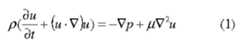

V - U = Q(2)
[052] and the convection-diffusion transport equation:

[053] where p, u, and p are the density, flow velocity and pressure of the liquid, and C and D are the concentration and diffusivity of the molecules in the liquid. At each time step, the flow u is first found independently of the concentration, which is then found using the computed flow. The boundary conditions are as follows. At the inlet, the flow velocity was set to 0.08cm/s for the forward flow and lO.lμm/s for the backward flow. These values agree with the average flow rates produced by the passive pump and by evaporation, experimentally observed and analytically calculated (see Appendix A). At the outlet we imposed zero normal stress, and at the channel walls we imposed the no-slip conditions (u = 0 ). For the convection-diffusion equation, constant concentration was set at the channel inlet and zero concentration at the channel outlet. No-flux conditions were imposed at all channel
walls . Table 1 in Appendix A summarizes the input parameters used for the numerical simulations. The channel geometry was set as 5cm x 1600μm x lOOμm and FTTC- Dextran was used as the model dye molecules. To quantify the simulation results with time, the concentrations were extracted from the centerline along the channel and normalized with the maximum concentration at the inlet of the channel.

Cytotoxicity testing
[054] HL-I cells (Cardiac muscle cell line) were cultured with medium containing 87% Claycomb Medium, 10% Fetal Bovine Serum (FBS), 1% Penicillin / Streptomycin, 1% Norepinephrine, and 1% L-Glutamine at 37 oC in a humidified 5% CO2 / 95% air incubator. To enhance the cell adhesion, the bottom glass slide was coated with a mixture of extracellular matrix (0.02% gelatin (w/w) and 5μg/mL fibronectin) after the top channel was bonded to the bottom glass slide. To seed the cells into the microfluidic device, the cells were trypsinized and seeded through the outlet port using dynamic seeding at a cell density of 2 x 10⁶ cells πiL-1 that allowed uniform cell distribution. Cells were cultured for 2 h to ensure attachment. The medium was then changed and 3 drops of 2μL medium containing 2OmM Alpha- cypermethrin were introduced by passive pumping and a concentration gradient was established by leaving the microfluidic device in the hood for 5min to allow for evaporation- induced backflow. The microfluidic device was then transferred to a humidified incubator where the concentration gradient of the toxin was stabilized and the cells were treated for 4h. Cell morphology and viability was characterized by peeling off the top channel and incubating the cells with live/dead dyes (2μL CaIc ein AM and 0.5μL Ethidium homodimer-1, Molecular Probes, California) in ImL DPBS for lOmin. ImageJ was used to quantify the fluorescence images of live-dead staining of the cells. At least three images were used for quantification of the cell viability.
Example 2
[055] In another example, a stable concentration gradient was produced using the process shown in Fig. 3. As described above, Fig. 3 shows a schematic diagram of the gradient generation and stabilization process: A) Microfluidic channel was first filled with DPBS; a large drop of DPBS was placed on the outlet opening and a small drop of the gradient material containing diffusible molecules was pipetted on the inlet opening, B) solution was introduced into the channel automatically by the passive-pump-induced forward-flow; C) a concentration gradient of molecules was generated during the evaporation-based backward flow; D) the gradient profile could be stabilized by stopping the evaporation, either by sealing the inlet with mineral oil or by maintaining the microfluidic device at 100% humidity. [056] In this example, the microfluidic channel was initially filled with DPBS, and a 200μL drop of DPBS was pipetted onto the outlet. A small drop of 2μL DPBS containing FITC- Dextran was then dropped onto the inlet (Fig. 3A) and entered the channel automatically due to the differential surface tensions between the drops (Fig. 3B). After the small drop entered the channel completely, a second drop was pipetted onto the inlet to continue the forward flow. In this example, three drops were sufficient for the fluid to reach the desired distance in the channel, in this example, the outlet end of the 5cm-long channel. The forward flow rate was ~lmm/s as measured experimentally and calculated analytically. Therefore, approximately one minute was required to introduce three drops of solution containing the fluorescent dye into the channel via the forward flow as shown in Fig. 4A. Following the forward flow, a backward flow was induced by the evaporation of the solution from the inlet. The concentration gradient of the fluorescent dye formed along the channel, which was parallel to the backward flow and moving backward toward the inlet, a shown in Fig. 3C and Fig. 4b. The backward flow rate was lO.lμm/s as measured experimentally and calculated analytically, which was significantly slower than the forward flow rate. The evolution of the centimeter-long concentration gradient that formed along the channel during the 50 min backward flow was quantified by measuring the fluorescent intensity along the channel and is shown in Fig. 4C, which was assumed to be proportional to the concentration of the fluorescent molecules. During the backward flow, the fluorescent dye and the concentration gradient moved backward toward the inlet, and the gradient steepened. [057] The gradient is generated by dispersion, the combined effect of convection and molecular diffusion, and flow reversal, which changes the direction of the parabolic flow shown in Fig. 5A. Concentration distributions at different locations along the channel at different times are shown in Fig. 5 B . The rapid forward flow generates a parabolic concentration profile as shown in Fig. 5B i. The backward flow then gradually flattens the parabolic profile and renders the concentration distribution laterally uniform as shown in Fig. 5B ii. A centimeter long concentration gradient with uniform cross- sectional distribution is formed after 16min of backward flow for molecule with a diffusivity of 1.7x10⁻⁶ cm2/s (i.e. FITC-Dextran) as shown in Fig. 5B iii. As the backward flow continues, the concentration forms a slightly inverted parabolic profile. However, since the backward flow is significantly slower than the forward flow, the uniformity of the concentration distribution was not significantly affected, and a relatively uniform concentration gradient moved backward toward the inlet as shown in Fig. 5B iv.
[058] The timescale for molecular diffusion across a distance L is L /(xD), where D is the molecular diffusivity. The timescales for vertical and horizontal mixing of FITC-Dextran across the lOOμm height and 1.6mm width of the channel are therefore 6 seconds and 25 minutes, respectively. Thus, the chemical concentration is essentially uniform vertically across the microchannel, and it suffices to consider only its horizontal variation, as we have done. The timescale for molecular diffusion across the width of the channel is significantly greater than the duration of the forward flow and commensurate with the timescale of the backward flow. It is therefore instructive to consider the role of the backward flow on gradient generation. After a concentration profile was produced by the forward flow, we compared the concentration profiles obtained after a given duration of backward flow with those obtained instead from the same duration of pure diffusion. The results indicate that the main role of backward flow is to spatially place the gradient. Moreover, the backward flow slightly elongates the gradient by l%-10%.
Stabilization of the concentration gradient
[059] To achieve the spatial and temporal control of the dynamic concentration gradients, a particular concentration gradient was stabilized using two methods to stop the flow. As shown in Fig. 3D and Fig. 6 A, evaporation from the inlet can be prevented either by sealing with mineral oil or by placing the microfluidic device in an environment with 100% humidity (water bath or cell incubator). The oil sealing approach could stabilize a particular concentration gradient profile for up to 4h before evaporation through the PDMS layer became noticeable (indicated by the small cavities in the fluorescence image in Fig. 6A, while a concentration gradient profile could be stabilized under 100% humidity for at least 12h.
[060] By preventing evaporation, the flow is stopped and spreading is due purely to (passive) molecular diffusion. The evolution of the concentration profile due only to molecular diffusion is shown over one day in Figs. 6B and 6C. The flow was terminated by setting equal the pressures at both the inlet and outlet of the channel. The concentration gradient after 12min of backward flow was used as the initial concentration profile. Simulations were run for two types of molecules with diffusion coefficients differing by an order of magnitude. The simulation results indicate that for large molecules with small diffusion coefficients (e.g. 10"7cm2/s), little change in the concentration gradient occurs due to molecular diffusion after one day. For smaller molecules with larger diffusion coefficients (e.g. 10"5cm /s), the effect of molecular diffusion on the concentration gradient profile became evident after 6h and approached equilibrium throughout the channel within one day. [061] Estimates can be made of the timescale over which the gradient is maintained, since exact analytical solutions are known for the diffusion equation for any initial concentration gradient. The exact solutions decay exponentially with rate constants approximately equal to JAD/L2, where L is the length scale of the concentration gradient and D is the molecular diffusivity. The concentration gradient is maintained to within 10% of its initial state over a time interval of 0.1L /( JΓD). Centimeter-long concentration gradients of chemicals with molecular diffusivities of 10"7cm2/s and 10"6cm2/s remain within 10% of their initial states over time intervals of approximately 28h and 2.8h, respectively. These results indicate that stable concentration gradients can be maintained for molecules over a wide range of diffusion coefficients for several hours.
Example 3 - Stabilized concentration gradient for cytotoxicity testing [062] In this example, the stabilized, spatially and temporally controllable concentration gradient technique is utilized for cytotoxicity testing. A cardiac muscle cell line (HL-I) is used to investigate the cytotoxicity of Alpha-cypermethrin, a cardiac toxin. Three drops of 2μL medium containing 2OmM Alpha-cypermethrin were loaded consecutively into the micro-devices with HL-I cells seeded along the channel. A concentration gradient of the toxin was established by evaporation when the micro device was left at ambient conditions for 5min (5min exposure does not cause severe damage to cell viability) and the gradient was stabilized when the micro device was transferred to the humidified incubator. HL-I cells exposed to the toxin concentration gradient for 4h exhibited distinguishable morphologies along the channel, with more severe effects observed in the regions containing higher concentrations of toxin. The drastic morphological change of HL-I cells exposed to various concentrations of toxin was also observed when the cytotoxicity testing was conducted with HL-I cells seeded in a 96-well plate. The cytotoxicity of the toxin gradient was further tested on the HL-I cells by conducting a live-dead assay. A correlation of cell viability was found with the toxin concentration gradient along the channel. According to the correlation between cell viability and morphology changes with respect to Alpha-cypermethrin concentration obtained from the toxicity testing on HL-I cells seeded in 96-well plates, the experimental conditions used in this example established a concentration gradient of the toxin from 12.5mM to OmM along the 5cm-length channel based on the assay conducted in this example. [063] According to the invention, the gradient generation process is highly reproducible at ambient conditions (i.e. 22 C, 30% relative humidity). Variations in temperature and humidity in the laboratory mainly affect the gradient generation process by slightly altering the backward flow rate induced by evaporation; their effects on the forward flow and the diffusion of the molecular are generally considered negligible.
[064] The flow is essentially fully developed Poiseuille flow throughout the rectangular channel. Regions of adjustment to the fully developed flow exist at the ends of the channel. However, based on the Reynolds numbers (0.1 and 0.001) of the forward and backward flows, the extent of these adjustment regions is short: approximately the channel height. Thus, throughout the channel the flow is essentially fully-developed Poiseuille flow. [065] The concentration gradient profile according to the present invention can be easily altered and controlled by choosing the initial analyte concentration in the applied drops and by manipulating the timing of the forward and backward flow. The factors affecting the flow properties, such as the fluid viscosity, the pressure difference between the inlet and outlet, the rate of evaporation and the geometry of the microfluidic channel affect the gradient generation.
[066] Second Embodiment
[067] Methods and systems according to an alternative embodiment of the invention utilize a pumping device, such a syringe pump, to drive fast alternating flows which continually lengthen the concentration gradient in the channel. This embodiment of the invention provides for rapidly generating multi- centimeter long concentration gradients along the channel in a simple and portable microfluidic device. Active pumping is provided to drive forward and backward flows in the channel. In addition, active pumping can be used to rapidly generate long cross gradients of two gradient materials in the channel of a simple and portable microfluidic device.
[068] Fig. 7 shows a diagram of a microfluidic device 700 according to an embodiment of the invention. The microfluidic device 700 includes a top portion 710 into which the microfluidic channel 716 is formed. The top portion 710 can be bonded to a bottom portion 720. The microfluidic device 700 also includes an inlet port 712 connected to one end of the microfluidic channel 716 and an outlet port 714 connected to the other end of the microfluidic channel 716. The inlet port 712 is connected by tubing to a pump 740, such as a syringe pump, which can inject and withdraw a predefined amount of the gradient material solution to the inlet port 712. In preparation of the concentration gradient, the channel can be filled with a buffered solution and optionally, a large drop 734 of the buffered solution can be placed on the outlet port 714. After the large drop 734 of buffered solution is placed on the outlet port 714, the pump 740 is operated or programmed to inject a predefined volume of the gradient material solution at a predefined flow rate into the inlet port 712, to induce a forward flow rate in the channel for a predefined time. According to one embodiment of the invention, the pump 740 is stopped for a predefined period of time to allow the diffusion to mix the solution vertically. After the predefined delay, the pump 740 is operated or programmed to withdraw a predefined volume of the gradient material solution at a predefined flow rate from the inlet port 712 to stretch the concentration gradient. The cycle comprising a forward flow, a delay and a backward flow can be repeated (with an optional delay in between) until the concentration gradient grows to fill the channel. After the last backward flow and an optional delay, an optional forward flow can be induced in the channel to increase the length of the gradient. The inlet port and optionally, the outlet port can be sealed to stop the growth and stabilize the concentration gradient.
[069] Figs. 8 shows a flow chart of the process of generating the concentration gradient in the microfluidic channel 716 according to an alternative embodiment of the invention. In accordance with the invention, the microfluidic channel 716, having an inlet port 712 and an outlet port 714, in which the concentration gradient is to be created, is provided at 802. The microfluidic channel 716 can be part of a microfluidic device 700 such as shown in Fig. 7. The microfluidic channel 716 is prefilled with a non-viscous solution, such as a buffer solution or culture medium, at 804. At 806, a large drop 734 of the non -viscous solution is optionally placed on the outlet port 714 and the pump 740 is operated or its program initiated to inject a predefined volume of gradient material solution into the inlet port 712 to cause a forward flow of the gradient material in the channel 716, from the inlet port to the outlet port. After the predefined volume of gradient material solution is injected into the inlet port 713, the pump 740 is stopped for a predetermined delay period to allow for diffusion, at 808. At the expiration of the delay period, the pump 740 is reversed (either manually operated or as part of a program) to withdraw a predetermined amount of gradient material solution at a predetermined flow rate, to cause a backward flow of the gradient material in the channel toward the inlet port 712, at 810. Depending on the desired length of the concentration gradient, cycle of forward flow, delay and backward flow, can be repeated using the same or different flow parameters (volume, flow rate and time delay) at 812 to grow the concentration gradient to the desired length. After the last backward flow (for example, 810), an optional delay (for example, 814) and, at 816, an optional forward flow can be caused by pumping a predetermined amount of gradient solution into the channel 716 to further stretch the concentration gradient. After the concentration gradient reaches the desired length, the inlet port and, optionally, the outlet port can be sealed (such as with oil or 100% humidity), at 818 to stabilize the concentration gradient in the channel 716.
[070] Fig. 10 shows a schematic for gradient generation and modes of spreading in channel flow. Fig. 1OA shows particles spreading due to hydrodynamic stretching. Fig. 1OB shows how diffusion suppresses longitudinal spreading. Fig. 1OC shows the effect of gravity on gradient material. Fig. 1OD shows advection and diffusion of solute dissolved in the flow, for high Pέclet number (high flow rate or small diffusivity) and low Pόclet number (low flow rate or high diffusivity).
[071] In accordance with this embodiment, fluidic shear-driven stretching, also known as hydrodynamic stretching, is the primary mode of gradient generation. A particle in the center of the channel moves faster than one at the wall and the two spread apart at a rate proportional to the maximum channel velocity. As shown in Fig. 1OA, a gradient forms in the laterally averaged concentration profile. Diffusion acts to suppress hydrodynamic stretching by reducing the mean variation in particle speeds slowly moving particles near the wall diffuse toward the centre and accelerate, while fast moving particles near the center diffuse toward the wall and decelerate as shown in Fig. 1OB. For dilute suspensions of micron sized and larger particles moving in viscous flows, diffusion is negligible. However, as shown in Fig. 1OC, negatively buoyant particles settle under gravity to the channel bottom, whereupon all particles experience the same low velocity and spreading ceases. Thus, high flow rates improve stretching at all scales: for molecules, high flow rates dominate diffusion which acts to suppress hydrodynamic stretching; for mi crop articles such as microbeads and cells, high flow rates are useful to spread the particles before they settle. In accordance with the invention, high-speed (mm/s) flow shear-driven stretching can be used to generate gradients of a wide range of gradient materials (e.g. molecules, cells and microbeads) along a simple microchannel.
[072] The spreading of gradient material in a microfluidic channel involves both hydrodynamic stretching (advection) and diffusion, a combined process known as dispersion as shown in Fig. 1OD. The Pέclet number Pe = UHZD specifies the ratio of the rates of transport by flow advection at speed U and molecular diffusion D in a channel of height H and ranges from approximately 400 to 4000 in our experiments. In the axial direction, transport is mainly due to advection; in the transverse direction, transport is due to molecular diffusion since the flow velocity is purely axial. A typical flow sequence to spread a diffusible species in a microchannel is illustrated in Appendix B, Fig. 1C and proceeded as follows. The transported species was introduced into one end of the channel and the flow began. The concentration profile was hydrodynamically stretched and the initially short, steep gradient in concentration spread (Appendix B, Fig ICi). The profile stretching was suppressed by lateral molecular diffusion, so that larger spreading was observed for larger Pέclet numbers. The flow was stopped before the gradient reached the end of the channel. At this point, as we explain shortly, it was advantageous to keep the fluid at rest for an order H KTCD) time (in our case ~ 5-30 s) to allow diffusion to completely mix the solution vertically (Appendix B, Fig. ICii). The flow was then reversed and stopped before the gradient reached the opposite end of the channel (Appendix B, Fig. ICiii). The cycle was repeated until a gradient of sufficient length was obtained. As the gradient grew and filled the channel, the flow segments became shorter. These short duration flows laterally smoothed the concentration profile by shortening the spatial lags between the wall and centreline concentration profiles.
[073] In a channel of uniform cross-section characterized by a height scale H and width scale W, where we assume without loss of generality that H ≤ W , three different regimes of dispersion exist: a short time regime t « H2 1 D where diffusion is not important, molecules follow the streamlines, and gradient growth is linear; an intermediate time interval H2 1 D « t « W2 1 D over which the molecules spread over the channel height; and a long time regime t »))W2 ID , called Taylor- Aris dispersion, over which molecules have sampled the entire channel cross-section. In one example, the channels are rectangular with a height H = 100 μm and width W= 2 mm, with molecules of diffusivity D ~ 10" to 10"e cm s" . Thus H2ZD is seconds to minutes and W2ZD is hours to days. Since the concentration gradients are generated in seconds to minutes, their evolution falls in the early to intermediate dispersion regime. Approximate theoretical descriptions valid for early, intermediate, and late times exist for many geometries, including rectangular channels, cylindrical tubes, and channels with smooth cross-sections. In these approximate theories, the cross-section ally averaged concentration has the classic erfc profile (Appendix B, IL3c) with a dispersivity D , which plays the role of an effective diffusivity, though orders of magnitude larger than the molecular diffusivity. The theories listed above give different forms for the dispersivity depending on the time regime and the geometry. All theories listed are for uni-directional flow; the effects of flow reversal can be computed numerically.
[074] To rationalize the experimental findings and to provide general experimental design criteria, a computational model was developed for the advection and diffusion of a diffusible species in sequences of forward and backward flow segments across a wide range of channel geometries and Pέclet numbers (Appendix B, II.3d). Dimensional analysis reduces the parameter space to four dimensionless parameters: W/H, Pe, Re, UH (Appendix B, ILl). In accordance with the invention, the Reynolds number Re=UHZv, which quantifies the relative magnitudes of fluid inertia and viscosity, is 0.1 or less. Thus, throughout the rectangular channel the flow is essentially fully developed laminar Poiseuille flow, a textbook exact solution to the Navier-Stokes equations governing the fluid flow (Appendix B, Fig. 5 and Supp. II.2). For this exact flow solution, which is independent of the axial coordinates, the convective derivatives in the Navier-Stokes equation vanish and hence so does the dependence on the Reynolds number. Since the flow velocity does not depend on the axial coordinate x, the effect of the channel length is merely to provide a stopping point once the gradient reaches the end of the channel. Thus, our computation model for the gradient evolution is characterized by only two parameters, W/H and Pe. Using the exact flow solution and for a wide range of parameter values, W/H = 1 to 20 and Pe = 100 to 104, a finite element code (Comsol AB) can be determined to solve the advection-diffusion equation in the microchannel on a rectangular grid (Supp. Fig. 2). In cases where the flow is off, molecular species spread via pure diffusion over the diffusive timescale τ = tD/H2, which has an analytical expression in the rectangular channel and may be readily calculated using discrete Fourier transforms (Appendix B, II.3a). Flow reversal is modelled by initializing the computational model with the concentration profile following the previous flow segment or pure diffusion segment and running the steady flow backwards. Further details including computational code and a sensitivity analysis are provided in Appendix B, II.3d. The resulting numerically computed concentration profiles were cross-sectionally averaged and the gradient length Δ was extracted. In this example, the gradient length Δ is defined as the distance between 10% and 90% of the maximum concentration, which captures the most linear, and therefore usable, portion of the concentration profile.
[075] Fig. 11 shows the generation of long-range molecular gradients. Fig.l IA shows long range molecular gradient generation in uni- directional flow: i) top-down view of fluorescent FITC-Dextran gradient and quantification along channel centerline at flow rates Q = 0.0092, 0.022, 0.035 ml/min; ii) simulation of gradient growth vs. time for various Pέclet numbers Pe and channel aspect ratios WlH; iii) gradient growth vs. time for experiments (mean flow speeds U = 2.5 (, \), 1.9 (α), 1.7 (x), 1.1 (*), 0.95 (!>), 0.62 (+), 0.58 (o) mm/s from left to right) and corresponding simulations (W/H=2Q, Pe = 1889, 1457, 1333, 884, 734, 476, 450 from left to right); iv) gradient length along centerline of channel after fluid travels x = 2.34 cm for experiments (o), simulation ( — vertically averaged centerline concentration, — cross-section ally averaged concentration), and fitting formula ( ); Fig. 1 IB shows long range molecular gradient generation in backward flow: top-down view of fluorescent FITC- Dextran gradient and quantification of centerline (C), wall (W), cross-sectionally averaged (A) gradient profiles, gradient length Δ and spatial lag σ. Fig. 11 C shows long range molecular gradient generation in alternating flow cycles: top-down view of fluorescent FITC- Dextran gradient and quantification along centerline, including gradient length Δ and spatial lag σ.
[076] In order to facilitate rapid gradient growth, higher flow rates dominate diffusion to generate longer gradients, even if the total distance the fluid moves along the channel is kept constant. This was quantified experimentally by producing gradients of FITC-Dextran with different flow rates, and theoretically with numerical simulations. Fluorescent images of the microchannel were captured at 5s intervals (Fig 1 IA i). Consistent with the definition above, in this embodiment, the gradient length Δ is defined as the distance over which the fluorescent intensity profile is between 10% and 90% of its maximum. Quantification of the fluorescent images illustrates that gradients grow faster and longer with higher flow rates. Our numerical simulations of gradient length support this conclusion (Fig HA ii). Higher Pέclet numbers are associated with faster gradient growth rates and longer gradients; the channel geometry has a secondary effect. The numerical predictions of gradient growth are in agreement with the experiments over a wide range of Pe (Figs. 1 IA iii-iv). The measured intensities were taken from above and were therefore vertically averaged, by definition. The numerical results were vertically averaged for comparison. In Figure 1 IA iii, the experimentally measured centreline gradient lengths compared well with predictions. To account for variable initial experimental gradient lengths (not controlled), the measurements were moved along the time axis so that the initial measurement coincided with the predicted gradient length profile. In Figure 1 IA iv, the numerical predictions of the centreline gradient length after the fluid moves a fixed distance Ut = 2.92 cm (simulation time f = tU/H = 234) also compare well with experimental data. In summary, the numerical results support the experimental finding that gradients grow faster at higher flow rates, and grow longer even when the different flows are allowed to move the same net distance down the channel. [077] For diffusible gradient materials in a finite channel, additional gradient growth can be obtained by subsequence backward and forward flow segments (Fig. 1 IB). Since the rapid gradient growth is due to high-speed flow rate shear-driven stretching, it is important to consider how the concentration profile shape and concomitant gradient length change when the flow is reversed. In the absence of diffusion, flow reversal would undo the hydrodynamic stretching and collapse the gradient. The effect of flow reversal on the gradient length was predicted numerically by reversing the flow after different durations of diffusion downtime followed the forward flow segment (Appendix B, Fig. 3). If the flow is reversed immediately without any diffusion downtime, gradients shrink as the hydrodynamic stretching of the previous flow segment is partially undone. With even brief diffusion downtimes, in particular those long enough to allow for vertical mixing, (t = QAH2ID ~ H2I(DK2) or τ = 0.1), the gradient shrinking is virtually eliminated for most channel cross-sections. The flow sequences used in the experiments involved multiple forward- backward flow cycles with 30 s diffusion downtimes between flow segments to allow for vertical mixing and to eliminate gradient shrinking. After four cycles (four forward segments and three backward segments), a 3 cm FITC gradient was obtained that was nearly laterally uniform (Fig. 11C). [078] Fig. 12 shows the generation of long-range gradient of particles, cells and materials. Fig. 12A shows an SEM image (with low and high magnification) of PEG-DA hydro gel gradient. Figs. 12B and C show an image of fluorescent particles (diameter 5 μm) and endothelial cells, respectively. Fig. 12D shows the quantification of the continuous variance in thickness of the hydrogel gradient. Fig. 12E shows the quantification of the relative density profiles of endothelial cells and fluorescent particles (with diameters of 5, 10 μm). [079] By combining material engineering technologies, the high-speed gradient generation method according to the invention was used to create material gradients of synthetic and natural polymers with controlled property variations. In each example, a concentration gradient of precursor solution of a material was first generated in accordance with one embodiment of the invention and then polymerized by the appropriate cross-linking method. Fig. 12A shows SEM images of the air-dried PEG-DA hydrogel gradient with a continuous variance in thickness. The concentration gradient of PEG-DA precursor solution was photopolymerized to form the hydrogel gradient. As quantified in Fig. 12E, the thickness of the dried hydrogel gradient gradually increased from ~10 μm in the region formed with 5wt% PEG-DA to ~40 μm in the region with 40wt% PEG-DA. In another example, thermally cross-linked collagen gradients were produced and visualized after free-drying. The porous 3D collagen mesh exhibited continuous changes of fibril density (Fig. 12B). [080] The gradient platform according to the present invention can also be used to produce material gradients of various mi crop articles. Using high flow speeds (mm/s), gradients of endothelial cells and 5 μm and 10 μm microbeads were generated along the channel (Fig. 12 C-E). The ability to rapidly generate nano/micro particle gradients may be useful to establish a controlled release system to deliver drugs with spatial variations. The cell gradient with controlled variations in cell density is potentially useful for generating bio-mimetic tissue constructs with heterogeneous cellular density and distribution (e.g. cartilage tissue). [081] Figs. 9 shows a flow chart of the process of generating a cross-gradient in the microti uidic channel 716 according to an alternative embodiment of the invention. In accordance with the invention, the microfluidic channel 716, having an inlet port 712 and an outlet port 714, in which a first concentration gradient has been generated, is provided at 902. The microfluidic channel 716 can be part of a microfluidic device 700 such as shown in Fig. 7. The microfluidic channel 716 includes a first concentration gradient, preferably produced in accordance with the invention. At 904, a large drop 734 of the second gradient material solution is placed on the outlet port 714. At 906, the pump 740 is operated or its program initiated to withdraw a predefined volume of solution from the inlet port 712 to inject the second gradient material solution into the outlet port and to induce the second gradient material to flow backward in the channel 116, from the outlet port to the inlet port. After the predefined volume of solution is withdrawn from the inlet port 712, the pump 740 is stopped, optionally, for a predetermined delay period, at 908. At 910, the pump 740 is reversed (either manually operated or as part of a program) to inject a predetermined amount of the solution (for example, a mixture of the first gradient material and the second gradient material in solution) into the inlet port at a predetermined flow rate, to induce the second gradient material to flow forward in the channel toward the outlet port 714. After the predeterimined volume of solution is injected into the inlet port 712, the pump 740 is stopped, optionally, for a predetermined delay period, at 912. Depending on the desired length of the concentration gradient, cycle of backward flow and forward flow, can be repeated using the same or different flow parameters (volume, flow rate and time delay) at 914 to grow the concentration gradient to the desired length. After the concentration gradient reaches the desired length, the inlet port and the outlet port can be sealed (such as with oil or 100% humidity), at 916 to stabilize the concentration gradient in the channel 716.
[082] The gradient platform according to the present invention allows cross- gradients to be formed by loading one species in one port, creating a single gradient on the forward flow, loading a second species in the opposite port and reversing the flow to create crossing gradients. Fig. 13 shows the generation of a cross gradient of FITC-Dextran and Rhodamine Dextran. Fig. 13A shows the merged fluorescence image of a cross gradient of FITC- Dextran (Green on right) and Rhodamine Dextran (Red on left). Fig. 13B shows the phase images (upper: lower magnification; lower: higher magnification) of SMC cultured on a substrate made from a composite material with HA-gelatin cross gradient. Fig. 13C shows the merged phase and fluorescence image of a cross gradient of 5μm fluorescent microbeads and non-fluorescent microbeads. Fig. 13D shows the quantification of the relative fluorescence of the FIT C-Dextran/Rhodamine Dextran cross-gradient and relative cell density on the composite materials with HA-gelatin cross-gradient.
[083] In one example, this method was used with four flow cycles to generate a 2 cm cross- gradient of the fluorescent dyes FITC-Dextran (mw 10KDa) and Rhodamine-Dextran (mw 1 OKDa) (Fig. 13A). The cross gradient approach according to the invention can be used to generate composite materials that can be used as multi-functional biomaterials with optimal biological, mechanical, and therapeutic properties for tissue engineering applications. As an example, the cross- gradient method according to the invention can be used to create a composite material that regulates cell attachment. Hyaluronic acid (HA) and gelatin regulate cell behaviour differently. HA is cell repellent, while gelatin is bio-active. Crossing gradients of the precursor solutions of methacrylated HA and gelatin were first formed and polymerized by UV cross- linking. Smooth muscle cells (SMCs) were cultured on the resultant HA-gelatin composite hydrogel to investigate the effect of the composite cross- gradient material on cell adhesion. After 24 h of incubation, the majority of attached SMCs were found on the gelatin dominant region and the number of attached cells gradually decreased along the composite cross gradient material as the ratio of HA increased (Fig. 13B,C). In addition to a cross gradient of polymers, a cross gradient of two types of microbeads can also be generated in a similar manner. In one example, Microbeads were loaded into opposing ports on successive flow segments with downtime in between to allow the first type of microbeads to settle. After one flow cycle, the two types of microbeads were well mixed with each other in different ratios along the channel, as shown in Fig. 13C, D. [084] To facilitate the design of gradient devices, the following approximate formula can be used to estimate gradient length,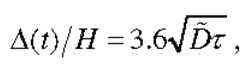 , where τ= tD/H2 is the dimensionless diffusive time and the dimensionless dispersivity is


[085] (see Supp. II.2c for details). The formula for D was originally found to be an excellent approximation for the dispersion between parallel plates, uniformly valid in time. An example of a table of the added fitting coefficients a and b is provided in Appendix C. For each W/H and Pe, values that best fit our numerical simulation of Δ(t) were chosen (Appendix B, Fig. 4). The maximum error between the numerical simulations and formula (1) is 7% over times 0 < tU/H < 1000. For large W/H, a and b approach 1, the case of the 2D infinitely wide channel. For large Pe, the growth rate becomes more linear, since the quantity ax is smaller. The numerical simulations are not sensitive to the grid resolution or the form of the initially smoothed step function (Appendix B, II.3d and Supp. Figs. 6, 7). Lastly, Excel and Matlab lookup tables for a and b are provided in Appendix B. The gradient length formula can serve as a tool for channel and flow design. As an example, we note that after a time t, the center of the gradient has moved a distance Ut and the gradient length is A(J), so the position of the tip of the gradient can be determined by Ut + A(t)/2, assuming the initial step profile was centered at x = 0. If the channel length is L and it is desired that the gradient be kept inside the channel, the flow duration must not exceed a time t* where Ut* + A(t*)/2 = L. Note that since diffusion suppresses gradient growth, the maximum distance particles of any type can move down the channel is 1.5Ut and hence A(J) < Ut. [086] While hydrodynamic stretching creates long gradients in seconds, the gradients produced may not be perfectly laterally uniform. The lateral (cross-sectional) non-uniformity is quantified by the distance σ between the x-locations of concentration c = 0.5 at the channel centre and at the wall. Appendix B, Figure 8A shows the center, wall, and laterally averaged concentration profiles over the initial forward flow segment. The profiles are more spread apart (higher σ) for higher flow rates; channel cross-section has a secondary effect (Appendix B, Fig. 8c). Initially σ grows linearly but may later grow more slowly due to diffusion. Diffusion alone can render the concentration profiles uniform over the long timescale WlD (Appendix B, Fig. 9). However, flow reversal combined with short diffusion downtimes offers a much faster approach. Appendix B, Figure 8b shows the center, wall, and averaged concentration profiles corresponding to those in Appendix B, Fig. 8a, following 30 s of pure diffusion downtime and a reverse flow segment. Numerical simulations of the backward flow illustrate that the separation σ decreases to 0 and then increases, as the hydrodynamic stretching of the previous flow segment is undone and then the profile is stretched in the opposite direction (Appendix B, Fig. 8d). If lateral uniformity is desired, the flow may be stopped when σ reaches zero. The longer the pure diffusion segments, the sooner σ reaches zero. However, since diffusion is relatively slow and the flows are relatively fast, lateral uniformity should be achieved primarily by the flow. As Appendix B, Fig. Ic iii illustrates, sufficient room must exist in the channel to move the gradient enough to reduce σ to zero. Thus depending on the application, an optimal flow sequence may involve a mix of flow segments devoted to growing the gradient and those devoted to improving lateral uniformity. Note that for no n- diffusible species, flow reversal will merely undo the hydrodynamic stretching and collapse the gradient, unless the particles are negatively buoyant and have settled, in which case flow reversal has no effect.
[087] In accordance with the invention, the channel size can affect the time required to generate a gradient of a given length Δ. In the absence of diffusion, the gradient length evolves as 1.2Ut, given above, which is independent of the channel dimensions provided the average flow speed U is kept constant. Generating a gradient of length Δ requires A/1.2U time. For non- diffusible species, a uniform gradient is formed once the particles settle to the channel bottom, and hence the settling time scales as the channel height. For diffusible species, increasing the smallest dimension of the channel, defined here as the height H, while keeping U constant increases the Pέclet number and enhances hydrodynamic stretching. However, achieving a uniform gradient requires lateral diffusive mixing. While flow reversal may be used to render the gradient uniform across the largest lateral dimension of the channel, defined here as the width, to avoid collapsing the gradient diffusive mixing must first complete across the height, which requires a time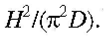 Thus while scaling up may enhance the hydrodynamic stretching, the total time to generate a uniform gradient scales as the channel height H for non-diffusible species and as H2 for diffusible species, where H is the smallest dimension of the channel.

[088] For completeness, we comment on the effects of other parameters on gradient evolution. The Reynolds number Re=UHZv and the scaled channel length UH do not directly affect the concentration profile and gradient evolution. The analytic solution for the fully developed flow profile has the special property that the convective derivatives in the Navier- Stokes equation vanish and hence so does the dependence on the Reynolds number. Moreover, since the flow solution is independent of the longitudinal coordinate x, the role of the channel length is merely to provide a stopping point once the gradient reaches the end of the channel. Thus while the channel length UH affects the choice of time sequence, it does not directly affect the concentration profile. Lastly, temperature affects gradient formation through its effect on the diffusion coefficient.
Materials:
[089] Poly(ethelyene glycol-diacrylate) with Molecular Weight 4000 is available from Monomer-Polymer & Dajac Labs. The photo-initiator (PI), 2-hydroxy-l-[4- (hydroxyethoxy)phenyl]-2-methyl-l-propanone (Irgacure D2959), is available from Ciba Geigy (Dover, NJ). Polyethylene microtubing (LD. 0.38 mm, O. D. 1.09 mm) is available from Intramedic Clay Adams (Becton Dickinson & Co, MD). Green Fluorescent FITC- microbead and non-fluorescent microbead solutions are available from Polysciences (Warrington, PA). Human Umbilical Vein Endothelial cells (HUVECs) and endothelial cell basal medium (EBM-2, Clonetics) supplemented with 0.5ML vascular endothelial growth factor (VEGF), 0.2ML hydrocortisone, 0.5ML epidermal growth factor (rhEGF), 0.5ML ascorbic acid, 2.0ML r-human fibroblast growth factor-B (rhFGF-B), 0.5ML heparin, 0.5ML recomb long R insulin- like growth factor (R3- IGF-I) and 0.5ML gentamicin sulfate amphotericin-B (GA-1000) are available from Lonza (Basel, Switzerland). All other reagents are available from Sigma- Aldrich (St. Louis, MO) unless specifically mentioned. [090] In accordance with one embodiment of the invention, the microfluidic device includes a microchannel was fabricated by standard soft lithography methods as described above. It includes a top Polydimethylsiloxane (PDMS) fluidic channel that was plasma bonded to a bottom glass slide. Preferably, the rectangular channel dimensions were lOOμm (height) x 2mm (width) x 50mm (length), although other channel dimensions can be used.
Generation of biomolecule gradient.
[091] In accordance with one embodiment of the invention, the microchannel was pre-filled with IX Dulbecco's Phosphate Buffered Saline (DPBS) solution. 1% wt fluorescein isothiocyanate-dextran (FITC-dextran) solution was introduced into the channel in one or more a cycle. Each cycle can include a forward flow, a delay, and a backward flow pumping sequence, for example: 4.67μl of the solution was pumped in (inducing forward flow) at 0.009 ml/min flow rate, wait 30 s of down time, and 2μl of the solution was withdrawn (inducing backward flow) at 0.022 ml/min flow rate. The cycle can be repeated as needed to increase the length of the concentration gradient, however, for this example, it was not needed. After the last cycle, there was a wait of 30 s for down time, and 1.34μl of the solution was pumped in (inducing forward flow) at 0.035 ml/min flow rate. The solution was pumped in and withdrawn using a syringe pump (World Precision Instruments Aladdin 1000, WPI, FL) and the flow rates were calibrated with a flow meter (from Gilmont Instrument, IL). The inlet and outlet ports can then be covered with oil or exposed to a 100% humidity environment to preserve the concentration gradient.
Generation of bead/cell gradient.
[092] In accordance with one embodiment of the invention, microbead stock solutions containing microbeads with diameters in 5.0 and 9.9 lμm (with a solid fraction of 0.1% w/w) were diluted 10 times in DPBS. The microfluidic device was the same as described above, a PDMS top portion bonded to a glass slide bottom portion. A syringe pump and flow meter were used to pump and withdraw the gradient material solution and measure the flow rates. In this embodiment, 6μL of the microbead solution was pumped into the channel at a rate of 0.035mI/min, followed by a 30s downtime before 4μL of the solution was withdrawn back into the tubing. 4μL of the fluid was pumped, then withdrawn, and finally pumped again into the channel with a 30s downtime between flow cycles.
[093] In an alternative embodiment of the invention, HUVECs were cultured in endothelial cell basal medium at 37° C in a humidified incubator. The protocol for generating cell gradients was similar to microbead gradients. The HUVEC medium was used in place of DPBS as the background solution and a medium containing HUVECs (5xlOe/ml) after trypsinization was used as the gradient material.
Generation of hydrogel gradient.
[094] In accordance with one embodiment of the present invention, a concentration gradient of hydrogel precursor solution (with high concentration of 40wt% PEG-DA in DPBS and 1% PI) was first generated at 0.022ml/min using the above-mentioned flow sequences for FITC- Dextran. To ensure the integrity of gradient in the hydrogel, 5wt% PEG-DA solutions were pre-filled in the channel. Upon photo-polymerization (UV exposure: lOmW/cm for 20s), the hydrogel precursor concentration gradient was cross-linked. For characterization, the resultant hydrogel was air-dried, cut with a scalpel blade to obtain a cross section, sputter- coated with gold and imaged using SEM (ULTRA 55, ZEISS). The thickness of the hydrogel was quantified relatively to the scale bar in the SEM image using ImageJ.
Generation of collagen gradient.
[095] In accordance with one embodiment of the present invention, the flow condition for generating PEG-DA hydrogel gradient was used to generate collagen concentration gradient (from 0.5mg/ml to 3.8mg/ml). Collagen fibers were formed upon gelation for 30min in the incubator (37 C). The device containing the collagen gradient was then pre-frozen at -20 C for lOmin and demoulded, exposing the collagen gradient. The collagen gradient was further frozen at -80 C for 2 hr and then freeze-dried in a lyophilizer. The morphology of the collagen gradient was visualized by SEM.
Generation of cross-gradient
[096] In accordance with one embodiment of the present invention, a concentration gradient was generated from a solution containing lwt% FITC dextran (MW: 10KDa) gradient material as described above. In accordance with the invention, the second gradient material, Rhodamine-Dextran (MW: 10KDa) is introduced at the outlet port by withdrawing a predefined quantity of solution from the inlet port. In this embodiment, 200μL Rhodamine- Dextran (MW: 1 OKDa) solution (lwt%) was pipetted onto the outlet port of the channel and 6μL Rhodamine-Dextran solution was withdrawn into the channel from the outlet at a flow rate of 0.022 ml/min with a syringe pump which was connected to the inlet of the channel. The solution (6μL) withdrawn into the tube was pumped back into the channel substantially immediately. This cycle of backward and forward flow induced by the pumping process was conducted for three times. The channel containing the cross- gradient of the double dyes was stabilized at least 30s before visualization. A series of continuous fluorescent images along the channel were taken using the green filter and red filter of the fluorescent microscope respectively and then were stitched together using Photoshop. The merged double dye cross- gradient was further quantified using ImageJ. To create the cross gradient of microbeads, 5μm diameter FIT C- microbeads and non-fluorescent beads were diluted 20 times. The similar protocol as for creating FITC-dextran/Rhodamine-Dextran was followed except that a higher flow rate of 0.035ml/min was used and only one flow cycle was conducted.
Generation of composite materials with cross- gradient of HA and gelatine. [097] In one embodiment of the present invention, Hyaluronic acid and gelatin were methacrylated to be photo- crosslinkable as described previously. 2wt% methacrylated HA solution (containing lwt% PI) was pre- filled into the channel and 2wt% methacrylated gelatin (lwt% PI) was added onto the outlet of the channel. HA and gelatin cross gradient was formed as mentioned above for FITC-dextran/Rhodamine-Dextran cross-gradient and stabilized upon photo-polymerization (UV exposure: lOmW/cm for 60s). Smooth muscle cells (SMC) were cultured in SMC basal medium (RPIM 1640, Gibco) at 37° C in a humidified incubator. Upon trypsinization, the cells were seeded in a density of lxlθ4cells/cm2 on the surface of HA-gelatin composite hydrogels. After 24h of incubation, the hydrogels were rinsed with sterile PBS for three times to wash away unattached cells and then fixed with 3.7% formaldehyde solution. A series of continuous phase contrast images along the channel were taken using microscope and then were stitched together. Cells were quantified by counting attached cell number using ImageJ.
[098] In accordance with the invention, the pump can be controlled by a controller, such as a computer, and the flow cycles can be programmed such that the flow cycles are completed automatically. Other types of pumps can be used. [099] Other embodiments are within the scope and spirit of the invention. Features implementing functions may also be physically located at various positions, including being distributed such that portions of functions are implemented at different physical locations. [0100] Further, while the description above refers to the invention, the description may include more than one invention.
Supplementary Material (ESI) for Lab on a Chip This journal is © The Royal Society of Chemistry 2008
Rapid generation of spatially and temporally controllable long range
concentration gradients in a microfluidic device
Yanan Du, Jaesool Shim, Mahesh Vidula, Matthew J. Hancock, Edward Lo, Bong Geun Chung, Jeffrey Borenstein, Donald Cropek, AIi Khademhosseini
Supplementary
• Input parameters for the computational simulations.
The diffusion coefficient is that for FITC-Dextran (MW 10KD) in water [250C]. The inlet velocity is obtained from the flow rates of the passive pump.

Table 1: Input parameters for computational simulations.
• Calculate the volumetric flow rate of the forward flow driven by the passive- pump:
We have developed a Maύab program to calculate the volumetric flow rate of the forward flow in the microchannel based on the analytical equations developed by Walker etaf: We found the solution to the following differential equation: Supplementary Material (ESI) for Lab on a Chip This journal is © The Royal Society of Chemistry 2008 where the radius of the drop R was determined by


To calculate the average flow rate in the channel, we first calculated the average volumetric flow rate, and then divided by the cross-sectional area of the channel. The average flow rate in channel was calculated as 0.08 cm/s.
M at lab program: function ypriine = volume(t,y) r = .O4; w= .01;
%w is the height of the channel g = .16;
%g is the width of the channel u = (8.90* 10Λ(-4));
%u is the viscosity of water
1 = 6;
%1 is the length of the channel z = (12*u* 10*l)/((wΛ3)*(g));
%z is the resistance of the channel a= 3*1^2; b = 6*y/pi; h = (l/6):t:(108:t:b+12:t:(12:t:aΛ3+81:t!bΛ2)Λ(.5))Λ(l/3)-(2:t:a)/((108:t:b+12:t:(12:t:aΛ3+81:t:bΛ2yϊ(.5)yϊ(l/3));
R = (3:t:y/pi+hΛ3):t:(l/3):t:(l/hΛ2); yprime = 1000*(l/z)*((-l)*98-145.6/R); end Supplementary Material (ESI) for Lab on a Chip This journal is © The Royal Society of Chemistry 2008
• Calculate the volumetric flow rate of the backward flow induced by evaporation:
The evaporation rate of water is calculated as the diffusion rate of water molecules coming out of water through the water/air interface (the boundary layer covering the water surface). The thickness of the boundary layer d is given by the following formulaJ:

4
The backward flow velocity can be expressed by

Where: d: the thickness of the boundary layer [cm]; v: kinetic viscosity of air [cm s" ];
Vmγ : air flow velocity [cm s" ];
V: velocity in the microfluidic channel [cm s" ];
PR : pump rate [cmJ s" ];
AE : area of the water/air interface [cm ];
M, P1 , D: molecular weight [g mol" ], density of the water [g cm" ], diffusion constant of water vapor in air [cm s" ]; pv , P3: vapor pressure of water [Pa], saturation vapor pressure of water [Pa];
R, T: ideal gas constant [cm Pa K mol ] and temperature [0C] (It is assumed that temperature is constant at the water/air interface); h, w: height and width of the microfluidic channel [cm]; r: radius of the port in the inlet [cm];
H: Relative humidity of the air Supplementary Material (ESI) for Lab on a Chip This journal is © The Royal Society of Chemistry 2008
The temperature dependence of D is known to be'i.
D oc T 1/2
(3)
The temperature dependence of v is known to be :
V oc T1 (4)
Clausius-Clapeyron equation is used to describe dependence of saturated water vapor pressure on temperature . :

According to equations (l)-(5), the velocity of backward flow can be expressed as:

Where C is a constant that combines the diffusion coefficient of water vapor in air, air flow velocity and proportional constants of Equations. (3), (4).
The backward flow rate at current operational condition (T=22°C, Η=30%) was lO.lμm s" . We also estimated the backward flow rate under other operational conditions (at other temperatures and relative humilities) based on equations (6), which were summarized in the table:

Assess the effects of backward flow on the resulting gradient Supplementary Material (ESI) for Lab on a Chip This journal is © The Royal Society of Chemistry 2008
To study the effects of the backward flow on the resulting concentration gradient, we compared the length of the gradient produced by either backward flow or pure diffusion. AU simulations started with the same initial concentration profile, produced by the forward flow, and were run with both low and high molecular diffusivities . In the first simulation, we measured the extent of the gradients produced at different times by the backward flow (Table 2), with effects from both convection and diffusion. In the second simulation, the extent of the gradient was measured after the same amounts of time of pure diffusion. The main difference between the two types of simulation is the location of the gradient: the backward flow moves the gradient back toward the inlet, while pure diffusion leaves it in place. This indicates the main role of the backward flow is to place the gradient. In both cases, diffusion acts to smooth the gradient. The results summarized in Table 2 also demonstrate that the backward flow slightly elongates the gradient by 1%- 10%, especially for cases with the low molecular diffusivity. This elongation may be due the flow-induced reversal of the parabolic shape of the concentration profiles.

Table 2: Comparison of the effects of backward flow and pure diffusion on the length of the gradient for high and low molecular diffusivity Supplementary Material (ESI) for Lab on a Chip This journal is © The Royal Society of Chemistry 2008
• Quantify the effect of diffusion on the change of the gradient profile
Following the slow backward flow stage, the flow is stopped and the concentration obeys the 3D diffusion equation subject to the boundary conditions of no-flux of chemical through the walls and ends of the channel. Exact solutions in terms of Fourier series are well known for any initial concentration. The chemical spreads and its concentration exponentially approaches a constant equilibrium value along the channel over a timescale J1* = L2 l\π2D), where L = X cm is the characteristic axial length and D is the molecular diffusivity. For example, for Z) = IO"7 and 10~6 cm /s, the gradient will decay over T* = 281 and 28 hours, respectively. To be more precise, note that the concentration c approaches its equilibrium constant value as exp(— TT2DtZL2) . Thus, to maintain the concentration gradient to within 10% of its initial state, we must have exp(-π2 Dt/ L2) > 0.9 . Rearranging yields / < ln(l/0.9)T* = 0.17 * . So, with
D = 10~7 and 10~e cm /s, the gradients remain within 10% of their initial states over time intervals of approximately 28 and 2.8 hours, respectively, in agreement with the numerical calculations.
• Cytotoxicity testing of Alpha-cypermethrin on HL-I cells cultured in 96-well microplate
HL-I cells were seeded into the 96-well microplate pre-coated with a mixture of extracellular matrices (0.02% gelatin (w/w) and 5 μg/mL fibronectin) at a density of 6.6x 10 cell/well and cultured in 100 μL Claycomb medium. The cells were exposed to Supplementary Material (ESI) for Lab on a Chip This journal is © The Royal Society of Chemistry 2008 medium containing various concentrations of Alpha-cypermethrin (from 12.5 πiM to 0 mM) for 5 min and 4 h respectively. For the 5 min cytotoxicity testing, the medium containing toxins was removed from the wells after 5 min and replaced with normal medium. After 4 h, the morphology and cell viability were tested. As shown in Fig. S l, after 4 h of exposure of HL-I cells to Alpha-cypermethrin, drastic changes of cell morphology were observed corresponding to the toxin concentration. We quantified cell viability after 4 h toxin exposure using image-based live/dead staining. In contrast, short- term exposure of HL-I cells to Alpha-cypermethrrn for 5 min did not induce observable changes of morphology or cell death (data not shown).
Supplementary Videos:
Video 1 : Video of experimental results of the time- lapse fluorescence images to show the dynamic concentration gradient generation during the backflow driven by evaporation.
Video 2: Video of simulation results to show the dynamic concentration gradient generation during forward flow when 3 drops of solution containing interested molecules were introduced into the channel.
Video 3: Video of simulation results to show the dynamic concentration gradient generation during the backward flow with a molecular diffusivity of 10" cm s" . Supplementary Material (ESI) for Lab on a Chip This journal is © The Royal Society of Chemistry 2008
Video 4: Video of simulation results to show the dynamic changes of concentration gradient driven by pure diffusion after the forward flow was stopped (with molecular ir} 1 diffusivity of 10" cm s" ).
Supplementary Material (ESI) for Lab on a Chip This journal is © The Royal Society of Chemistry 2008
Supplementary figures:

Figure. S l: Cytotoxicity testing of Alpha- cypermethrin on HL-I cells cultured in 96- well microplate: A) HL-I cell morphology; B) live/dead assay of HL-I cell after exposure to various concentrations of Alpha-cypermethrin for 4h (scale bar: 400μm). Supplementary Material (ESI) for Lab on a Chip This journal is © The Royal Society of Chemistry 2008

Figure. S2: Top-down view of the simulation results of the dynamic changes of concentration gradient driven by pure diffusion after the forward flow was stopped (with a molecular diffusivity of 1.7x10" cm /s).
References:
1. B. G. Chung, F. Lin and N. L. Jeon, Lab on a chip, 2006, 6, 764-768.
2. G. M. Walker and D. J. Beebe, Lab on a chip, 2002, 2, 131-134.
3. H. Kazuo, T. Satoko and A. Youko, Journal of Applied Physics, 1993, 73, 7395- 7401.
4. F. Heuck, T. Hug, T. Akiyama, P. L. T. M. Frederix, A. Engel, A. Meister, H. Heinzelmann, N. F. d. Rooij and U. Staufer, Microelectron. Eng., 2008, 85, 1302- 1305.
5. D. Bolton, Monthly weather review, 1980, 108, 1046-1053.


II. SUPPLEMENTARY METHODS ILl Dimensional analysis
To reduce the complexity of the problem and identify the salient dimensionless parameters, we non- dimensionalize the system. The physical system has eight parameters, Q (flow rate), L (channel length), W (channel width), //(channel height), p (fluid density), V (fluid viscosity), D (diffusivity of the species), and Ctnax (the maximum concentration). The average speed U in the channel is given by QZ(WH). We divide all lengths by//, speeds by U, time by HIU, and concentrations bycrnaκ. The dimensionless system has four parameters: Pe = UHID (Peclet number), Re = UH/v (Reynolds number), WIH (channel cross- section aspect ratio), ////(scaled channel length).
11.2 Fully developed channel/pipe flow
The flow is assumed steady and is characterized by the channel cross-sectional aspect ratio WIH and the Reynolds number Re which quantifies the relative magnitudes of fluid inertia versus viscosity. In the regime of interest, Re is approximately 0.1 or less; the flow is dominated by viscosity. Low Reynolds number flows in channels and tubes become fully developed (i.e. independent of the axial coordinate) approximately within the distance of the smallest cross-sectional dimension of the channel [H/2 for rectangular channels of height H, d/2 for tubes of radius d).(26) Fully developed steady flow in channels whose height H, width W, and length / are orders of magnitude apart, H <ϋ W <£ L , is well approximated bythe 2D parabolic profile between parallel plates, (27) in dimensionless form for -0.5 < z < 0.5, where the sign indicates the flow direction. Fully developed steady flow in rectangular pipes of arbitrary cross-section is given in dimensionless form by(26, 28, 29)


11.3 Mass transport
For the steady uni-directional channel flows given in (1) - (3), the mass transport is governed by the dimensionless advection-diffusion equation where V is the dimensionless Laplacian operator. In circular pipes with axisymmetric flow (3) and inlet/outlet concentrations, the concentration in the pipe is axisymmetric and is modeled by (4) in cylindrical coordinates [rjc] with the axisymmetric cylindrical polarform of the Laplacian V .

11.3a Diffusion
In the limit of pure diffusion [u = Q), (4) becomes the well-known diffusion equation where the dimensionless diffusive timescale is τ = t/Pe = tDIH . (5) admits exact solutions in rectangular channels and pipes for any initial concentration and for various steady boundary conditions on the channel sides. (31, 32) For our rectangular channels that have no-flux conditions at the walls (z= 1/2 ory = WI(THf) and symmetry planes (z = 0 oxy = 0) and the Dirichlet conditions c = 1 at the inlet (z = 0) and c = 0 at the outlet (z = L/H), the solution to (5) is


Both~cv (x, y,T) and c(x,τ) are computed by first computing cjm n as above and then using inverse transforms or calculating the sum directly (Supp. Code Example 1). ll.3b Convection / Hydrodynamic Stretching
In the limit of zero diffusion ( Pe = °°), spreading is due only to convection, also known as flow advection or hydrodynamic stretching. In this zero diffusion limit, the solution to (4) is c = f(x — u(y,z)t,y,z) where c =flxy,z) is the initial concentration. Particles move different speeds at different elevations and a gradient forms in the vertically averaged concentration profile. The gradient may be found for general velocity and initial concentration profiles by numerically averaging across the channel. We consider the simple case of parabolic flow, Eq. (1), which holds in the central region of the channel, and a unit step in initial concentration, β^x,y^) = Hv(x). In this case, the cross-sectionally averaged concentration is given by(33)


From (10), c = CC at the position xa(f) = 3t(l-CC2)/2 . The length of the front is given by xo(t)-x1(t) = 3Ut/2 =umiKt (11)
This result has been given previously for circular tubes( 34, 35) where the length of the front is 2Ut. The length of the gradient is given by

II.3c Taylor dispersion
The advection and diffusion of a transported species (chemical or particle) in a tube or rectangular channel was first reported in the 1950s by Taylor(35, 36) and Aris,(37, 38) and is now a textbook example(27, 34, 39, 40) known alternately as flow shear-driven, Taylor, or Taylor-Aris dispersion. Approximate theoretical descriptions valid for early, intermediate, and late times exist for many geometries, including rectangular channels, (28, 41) cylindrical tubes, (42) and channels with smooth cross-sections. (20, 21) In these theories, the cross-sectionally averaged concentration profile is given approximately by where + indicates the flow direction, and De# is the dimensionless dispersivity, or dispersion coefficient, which takes different forms for different geometries and time regimes. Rearranging (13) gives the length Δ(/) of the linear portion of the gradient, here defined as the distance between C^ = 0.9 and Z7 = 0.1,
 For cylindrical tubes, (42)
 where τ = t/Pe isthe diffusive timescale and μn are the positive roots of J1(^Zn) = 0 forn = 1,2,3... For the flow between parallel plates (infinitely wide channel), an approximate formula valid to within 1% of the full series result is'43' given in Eq, (2) in the main text. In the limit of small τ and for large Pe, De^and Δ grow linearly in time, consistent with mass transport by convection alone. A sophisticated power series formula for the dispersivity Z)e// exists for rectangular channels, " although during intermediate times it depends on the initial concentration distribution. II.3d Numerical simulation of mass transport in microchannels


The analytic estimates listed above for dispersivity and gradient length are valid for uni-directional flow. Numerical simulations are required to predict the effects of flow reversal on the concentration profile. The numerical finite element package Comsol 3.4 was used to solve (4) subject no-flux boundary conditions at walls [y = WKlH) or z = 1/2) and symmetry planes [y = 0 or z = 0) and the Dirichlet conditions c = 1 at the inlet (x = 0) and c = 0 at the outlet (x = L/H) (Supp Fig. IB). The concentration profile and flow for circular tubes is assumed axisymmetric. The initial condition was chosen to be a smoothed step function (flc2hs in Comsol) in x of dimensionless width 10 or 20. A rectangular mesh of the computational domain, the upper quadrant of the channel, was employed with 100, 20, and 11 gridpoints in x, y, and z, respectively, with more gridpoints near the walls (Supp. Fig. 2). The GMRES linear system solver was used. The Courant-Friedrichs-Lewy (CFL) time step condition(45) was used to guarantee stability. Our Comsol code required to set up the geometry, mesh, model and run a basic simulation is given in Supplementary Code Example 3.
The gradient length Δ, position of c = 0.5 , X50, and the spatial lag σ were insensitive to the precise shape of the initial smoothed step function. The width and shape of the step function were altered (Supp. Code Ex. 2) and did not affect the evolutions of the gradient length or center position after brief initial transient times (Supp. Fig. 6). Also, the grid resolution was chosen sufficiently fine to produce results independent of the grid spacing. Simulations run with normal double resolution produced nearly identical gradient lengths Δ (to visual inspection) and the differences in the gradient center position .V50 and the spatial lag σ were within 0.11% and 3,2%, respectively, of the gradient length (Supp. Fig. 6). In other words, our grid resolution was sufficiently fine.

Simulations were run both in the "fixed frame" and "moving frame" with a fixed mesh. In fixed frame simulations, the chemical gradient moves down the channel with the flow and the flow is stopped before the gradient reaches the end of the channel. For much of this evolution, c = 0 or l in the majority of the channel. To improve accuracy for a given amount of desktop computer memory, we have also performed simulations in a frame moving with the dimensionless mean speed 1. We employed the moving coordinate ξ = x — t and an expanding computational domain (in the x-direction) with a fixed number of gridpoints. For this type of simulation, u — 1 and ξ replace u and x in (4), including the Laplacian V . The grid structure is identical for both types of simulation, but the grid spacing in the x- direction increases as the domain is expanded. Initially, the length of the computational domain was 100 and the initial concentration (smoothed step function) was centered. As time progressed and the gradient grew, the length of the computational domain was increased to fully contain the gradient and keep the concentration near the inlet above 0.995 and that near the outlet below 0.005. For higher Peclet numbers the length of the domain was increased at greater rates. The channel cross-section mesh was kept constant throughout. To produce user-friendly formulas to estimate gradient length, we collapse our simulation output onto formulas (1) in the main text, with dispersivity of the form of (2) in the main text,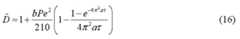

The fitting coefficients a and b were chosen for each WIH and Fe for best fit with our numerical simulations of Δ(/) (Fig S.4). The maximum error was 7% over times 0 < tU/H < 1000. For large WIH, a and b approach 1, the case of the 2D infinitely wide channel. Lastly, Excel lookup tables (fit.xls) forα and b are provided with the Supplementary Information. Since our simulation output is not sensitive to the form of the initial concentration profile, neither should be our results for a and b.
II.3e Diffusivity of particles
Particles spread in viscous flows due to Brown ian diffusivity (DB = kT/(6π\ia)), particle interaction and inertia I lift. (46) For particle diameters larger than 1 μm moving in a flow with shear rate γ, the Brownian diffusivity is generally negligible, since(46) the particle Peclet number .Pep = 'yμα JkT » 1. lnertial lift is negligible in microchannel flows where viscous forces dominate (Re ≤ 1). Two forms of particle interaction are possible: (i) self-diffusion, due solely to particle collisions and (ii) gradient diffusion, where particles experience greater resistance when moving into regions of higher particle concentration compared with those of lower concentration. For dilute suspensions, the gradient diffusion is negligible and the self-diffusivity is(47) D = O.Sja φ where φ is the volume fraction. The shear rate of flow between fixed parallel plates is γ= UfH. For the 5, 10 μm microbeads in our experiments, the concentration (w/w) was 10"3 and 2.65xlO"3, respectively, the density was 1.05 g/ml, the volume fraction was 9.52xlO"4 and 2.52xlO"3 (vol/vol), respectively, and the average flow speeds were 2.1 mm/s and 3.2 mm/s. Since the height of the channel is 100 μm, the self-diffusivity is then D = 6.OxIO"13 cm2/s and 2.SxIO"11 cm2/s, respectively. Since the standard molecular diffusivities are of the order 10"6 cm2/s (small molecule) and 10"7 cm2/s (large molecule), the self-diffusivities of the microbeads are negligible and the particles spread from hydrodynamic stretching only. The cell concentration was 5.OxIO6 cells/ml and the average flow speed was 3.2 mm/s. Assuming a cell diameter of 10 μm gives D=S1OxIO"11 cm2/s, again orders of magnitude smaller than that for molecules.
11.4 Experimental methods
Image analysis of FITC- Dextr an biomolecule gradient. Fluorescence images of the F ITC-De xt ran gradient along the channel under different flow rates (repeated at least three times) were captured at 5 s intervals with a 0.8 s exposure time using a Kodak Gel Logic 100 Imaging System and the fluorescence intensity along the channel was quantified with NIH ImageJ software. Following Goulpeau et a!., (20) images of the channel filled with DPBS (background = S) and filled with the FITC-Dextran solution (maximum = M) were used to calibrate the intensity signal (S) by the formula (S-B)I(M-B) to remove the spatial heterogeneities induced by the fluorescence excitation source and the variable translucence of the PDMS.
Image analysis of bead/ cell gradient. Images were captured along the length of the channel during the course of the experiment by using a florescence microscope (Nikon, USA) with 2X or 1OX objectives. The images containing the microbeads/cells in the entire microfluidic channel were generated by stitching 7 images of the adjacent 0.5 cm segments of the channel using Adobe Illustrator. Microbeads or cells in each image were counted using the particle counting function in ImageJ, Particle counts in each image were normalized by the maximum particle count in a given segment for comparison across different experiments.


1. Chen H, He Z, Bagri A & Tessier-Lavigne M (1998) Semaphorin-neuropilin interactions underlying sympathetic axon responses to class III semaphorins. Neuron 21:1283.
2. Foxman EF, Kunkel EJ & Butcher EC (1999) Integrating conflicting chemotactic signals: the role of memory in leukocyte navigation. J Cell Biol 147:577.
3. Wu H, Huang B & Z are RN (2006) Generation of complex, static solution gradients in microfluidic channels. JAm Chem Soc 128:4194-5.
4. Boyden S (1962) The chemotactic effect of mixtures of antibody and antigen on polymorphonuclear leucocytes. J Exp Med 115:453.
5. Zigmond SH (1977) Ability of polymorphonuclear leukocytes to orient in gradients of chemotactic factors. J Cell Biol 75:606.
6. Ming GL, et al. (2002) Adaptation in the chemotactic guidance of nerve growth cones. Nature 417:411.
7. Chung BG, Lin F & Jeon NL (2006) A microfluidic multi-injector for gradient generation. Lab Chip 6:764-768.
8. Mao H, Cremer PS & Manson MD (2003) A sensitive, versatile microfluidic assay for bacterial chemotaxis. Proc Nail Acad Sci USA 100:5449.
9. Kim D, Lokuta MA, Huttenlocher A & Beebe DJ (2009) Selective and tunable gradient device for cell culture and chemotaxis study. Lab Chip 9:1797-1800.
10. Li CW, Chen R & Yang M (2007) Generation of linear and non-linear concentration gradients along microfluidic channel by microtunnel controlled stepwise addition of sample solution. Lab Chip 7:1371-1373.
11. Mosadegh B, et al. (2007) Generation of stable complex gradients across two-dimensional surfaces and three-dimensional gels. Langmuir 23:10910.
12. Paliwal S, et al. (2007) MAPK-mediated bimodal gene expression and adaptive gradient sensing in yeast. Nature 446:46-51.
13. Cooksey GA, Sip CG & Folch A (2009) A multi-purpose microfluidic perfusion system with combinatorial choice of inputs, mixtures, gradient patterns, and flow rates. Lab Chip 9:417-426.
14. Irimia D, Geba DA & Toner M (2006) Universal microfluidic gradient generator. ,4Ma/ Chem
15. Kamholz AE, Weigl BH, Finlayson BA & Yager P (1999) Quantitative analysis of molecular interaction in amicrofluidic channel: the T-sensor. Anal Chem 71:5340.
16. Lin F, et al. (2004) Generation of dynamic temporal and spatial concentration gradients using microfluidic devices. Lab Chip 4:164-167.
17. Jeon NL, et al. (2002) Neutrophil chemotaxis in linear and complex gradients of interleukin-8 formed in amicrofabricated device. Nat Biotechnol 20:826-830.
18. Lee K, Kim C, Aim B &Panchapakesan R (2009) Generalized serial dilution module for monotonic and arbitrary microfluidic gradient generators. Lab Chip 9:709.
19. Javier A, Morrow J & Locascio LE (2009) The microfluidic palette: A diffusive gradient generator with spatio-temporal control. Lab ChipDOl: 10.1039/b902113b.
20. Goulpeau J, Lonetti B, Trouchet D, Ajdari A & Tabeling P (2007) Building up longitudinal concentration gradients in shallow micro channels. Lab Chip 7:1154-1161.
21. Ajdari A, Bontoux N & Stone HA (2006) Hydrodynamic dispersion in shallow microchannels: the effect of cross-sectional shape. Anal Chem 78:387-392.
22. Du Y, et al. (2009) Rapid generation of spatially and temporally controllable long-range concentration gradients in amicrofluidic device. Lab Chip 9:761-767.
23. Kang T, Han J & Lee KS (2008) Concentration gradient generator using a con vective -diffusive balance. Lab Chip 8:1220-1222.
24. Fawcett JS, Sullivan JV, Chidakel BE & Chrambach A (1988) A motor- driven syringe-type gradient maker for forming immobilized pH gradient gels. Electrophoresis 9:216-221. 25. DeLong SA, Moon JJ & West JL (2005) Covalently immobilized gradients of bFGF on hydrogel scaffolds for directed cell migration. Biomaterials 26:3227-3234.
26. White FM (1991) Viscous fluid flow (McGraw-Hill, New York).
27. Bird RB, Stewart WE & Lightfoot EN (2002) Transport phenomena (Wiley, Madison, USA).
28. Chatwin PC & Sullivan PJ (1982) The effect of aspect ratio on longitudinal diffusivity in rectangular channels. J Fluid Mech 120:347-358.
29. Happel J & Brenner H (1991) Low Reynolds number hydrodynamics: with special applications to particulate media (Kluwer, Boston).
30. Acheson DJ (1990) Elementary fluid dynamics (Oxford University Press, USA.
3 ] . Myint-U T & Debnath L (2007) Linear partial differential equations for scientists and engineers (Birkhauser, Boston).
32. Du Chateau P & Zachmann DW (1986) Schaum 's outline of theory and problems of partial differential equations (McGraw-Hill, New York).
33. Gill WN & Guceri U (1971) Laminar dispersion in Jeffery-Hamel flows: Parti. Diverging channels. ALChE J 17.
34. Probstein RF (1994) Physicochemical hydrodynamics: an introduction (Wiley-Interscience.
35. Taylor GI (1953) Dispersion of soluble matter in solvent flowing slowly through a tube. Proc R Soc London, A 219:186-203.
36. Taylor GI (1954) Diffusion and mass transport in tubes. P Phys Soc LondB 67:857-869.
37. Aris R (1959) On the dispersion of a solute by diffusion, convection and exchange between phases. Proc R Soc London, ,4:538-550.
38. Aris R (1956) On the dispersion of a solute in a fluid flowing through a tube. Proc R Soc London, A:67-77.
39. Tabeling P & Cheng S (2005) Lntroduction to microfluidics (Oxford University Press, USA.
40. Brenner H & Edwards DA (1993) Macrotransport processes (Butterworth-Heinemann, Boston).
41. Doshi MR, DaiyaPM & Gill WN (1978) Three dimensional laminar dispersion in open and closed rectangular conduits. Chem E 'ng Sci 33 :33.
42. Van den Broeck C (1982) A stochastic description of longitudinal dispersion in uniaxial flows. PhysicaA 112:343-352.
43. Haber S & Mauri R (1988) Lagrangian approach to time-dependent laminar dispersion in rectangular conduits. Part 1. Two-dimensional flows. J Fluid Mech 190:201-215.
44. Mauri R & Haber S (1991) Time-dependent dispersion of small particles in rectangular conduits. SLAMJ ApplMath 51:1538-1555.
45. Courant R, Friedrichs K & Lewy H (1967) On the Partial Difference Equations of Mathematical Physics. LBM Journal of Research and Development 11:215.
46. Chapman BK & Leighton DT (1991) Dynamic viscous resuspension. Lnt J Multiphas Flow 17:469-483.
47. Leighton D & Acrivos A (1987) Measurement of shear-induced self- diffusion in concentrated suspensions of spheres. J Fluid Mech 177:109-131.

Claims
1. A method of creating a concentration gradient in a microfluidic device, the device comprising a microfluidic channel formed in a substrate material connecting an inlet port and an outlet port, the method comprising: filling the microfluidic channel with a non-viscous solution; inputting into the inlet port, a predefined amount of gradient material solution, and causing a passive pump-driven forward flow in the microfluidic channel; and evaporating the gradient material solution from the inlet port and causing an evaporation- driven backward flow; and sealing the inlet port.
2. The method according to claim 1 wherein applying a predefined amount of the gradient material solution includes applying one or more drops of the gradient material solution to the inlet port.
3. The method according to claim 1 wherein evaporating the gradient material solution includes allowing the gradient material solution to evaporate from the inlet port.
4. The method according to claim 1 wherein evaporating the gradient material solution includes reducing the pressure in an area adjacent to the inlet port.
5. The method according to claim 1 wherein evaporating the gradient material solution includes increasing the temperature in an area adjacent to the inlet port.
6. The method according to claim 1 wherein the non- viscous solution is a buffered solution.
7. The method according to claim 1 further comprising applying a predefined amount of non-viscous solution to the outlet port prior to inputting a predefined amount of gradient material solution to the inlet port, whereby a large drop of non- viscous solution forms over the outlet port.
8. The method according to claim 1 wherein the gradient material solution includes gradient material selected from the group including diffusible molecules, biologic molecules, polymers, beads, particles and cells.
9. The method according to claim 1 wherein evaporating the gradient material from the inlet port is allowed to occur for at least 20 minutes before sealing the inlet port.
10. A microfluidic device comprising a concentration gradient formed from a concentration gradient material according the method of claim 1.
11. A method of creating a concentration gradient in a microfluidic device, the device comprising a microfluidic channel formed in a substrate material connecting an inlet port and an outlet port, the method comprising: filling the microfluidic channel with a non-viscous solution; injecting a gradient material solution into the inlet port according to at least one alternating flow cycle, the flow cycle comprising: pumping a predefined amount of gradient material solution into the inlet port at a first predefined flow rate and causing a forward flow of the gradient material solution in the microfluidic channel; waiting a predefined delay; withdrawing a predefined amount of the gradient material solution from the inlet port at a first predefined withdrawal flow rate and causing a backward flow of the gradient material solution in the microfluidic channel; and sealing the inlet port.
12. The method according to claim 11 further comprising, prior to sealing the inlet port, waiting a predefined delay; and pumping a predefined amount of gradient material solution into the inlet port at a first predefined flow rate and causing a forward flow of the gradient material solution in the microfluidic channel.
13. The method according to claim 11 comprising a second flow cycle prior to sealing the inlet port, the second flow cycle comprising: pumping a second predefined amount of gradient material solution into the inlet port at a second predefined flow rate and causing a forward flow of the gradient material solution in the microfluidic channel; waiting a predefined delay; and withdrawing a second predefined amount of the gradient material solution from the inlet port at a second predefined withdrawal flow rate and causing a backward flow of the gradient material solution in the microfluidic channel.
14. The method according to claim 13 comprising a third flow cycle prior to sealing the inlet port, the third flow cycle comprising: pumping a third predefined amount of gradient material solution into the inlet port at a third predefined flow rate and causing a forward flow of the gradient material solution in the microfluidic channel; waiting a predefined delay; and withdrawing a third predefined amount of the gradient material solution from the inlet port at a third predefined withdrawal flow rate and causing a backward flow of the gradient material solution in the microfluidic channel.
15. The method according to claim 11 further comprising applying a predefined amount of non-viscous solution to the outlet port prior to injecting a predefined amount of gradient material solution to the inlet port according to the at least one flow cycle, whereby a large drop of non -viscous solution forms over the outlet port.
16. The method according to claim 11 wherein the microfluidic device includes a top portion and a bottom portion and the method further comprises applying ultraviolet light energy to the gradient material to solidify the gradient material in the microfluidic device and removing the top portion of the microfluidic device to expose the solidified gradient material.
17. The method according to claim 11 wherein the microfluidic device includes a top portion and a bottom portion and the method further comprises freezing the gradient material to solidify the gradient material in the microfluidic device and removing the top portion of the microfluidic device to expose the solidified gradient material.
18. The method according to claim 11 wherein the length of the concentration gradient is determined as a function of a flow speed at which the gradient material flows is induced to flow in the microfluidic channel and an amount of time the gradient material is allowed to flow at the flow speed.
19. A microfluidic device comprising a concentration gradient formed of a gradient material according to the method of claim 11.
20. A method of creating a cross-concentration gradient in a microfluidic device, the device comprising a microfluidic channel formed in a substrate material connecting an inlet port and an outlet port, the method comprising: providing a microfluidic device having a concentration gradient of a first gradient material in the microfluidic channel; applying a predefined amount of a second gradient material solution to the outlet port, whereby a large drop of the second gradient material solution forms over the outlet port; withdrawing a predefined amount of solution from the inlet port at a predefined withdrawal flow rate and causing the second gradient material solution to enter the outlet port and causing a backward flow of the second gradient material solution from the outlet port to the inlet port in the microfluidic channel; and pumping a predefined amount of solution into the inlet port at a predefined flow rate and causing a forward flow of the second gradient material solution from the inlet port to the outlet port in the microfluidic channel.
21. A microfluidic device comprising a cross-concentration gradient formed of a first gradient material and a second gradient material according to the method of claim 20.
Priority Applications (1)
| Application Number | Priority Date | Filing Date | Title |
|---|---|---|---|
| US13/129,190US20110300570A1 (en) | 2008-11-14 | 2009-11-16 | Method and system for generating spatially and temporally controllable concentration gradients |
Applications Claiming Priority (2)
| Application Number | Priority Date | Filing Date | Title |
|---|---|---|---|
| US11453908P | 2008-11-14 | 2008-11-14 | |
| US61/114,539 | 2008-11-14 |
Publications (2)
| Publication Number | Publication Date |
|---|---|
| WO2010057078A2true WO2010057078A2 (en) | 2010-05-20 |
| WO2010057078A3 WO2010057078A3 (en) | 2010-09-02 |
Family
ID=42170764
Family Applications (1)
| Application Number | Title | Priority Date | Filing Date |
|---|---|---|---|
| PCT/US2009/064555WO2010057078A2 (en) | 2008-11-14 | 2009-11-16 | Method and system for generating spatially and temporally controllable concentration gradients |
Country Status (2)
| Country | Link |
|---|---|
| US (1) | US20110300570A1 (en) |
| WO (1) | WO2010057078A2 (en) |
Cited By (11)
| Publication number | Priority date | Publication date | Assignee | Title |
|---|---|---|---|---|
| WO2013134741A3 (en)* | 2012-03-08 | 2013-12-19 | Cyvek, Inc. | Methods and systems for manufacture of microarray assay systems, conducting microfluidic assays, and monitoring and scanning to obtain microfluidic assay results |
| CN103941022A (en)* | 2014-03-07 | 2014-07-23 | 大连理工大学 | Microfluidic three-dimensional flow delay control unit |
| US9229001B2 (en) | 2009-11-23 | 2016-01-05 | Cyvek, Inc. | Method and apparatus for performing assays |
| US9651568B2 (en) | 2009-11-23 | 2017-05-16 | Cyvek, Inc. | Methods and systems for epi-fluorescent monitoring and scanning for microfluidic assays |
| US9700889B2 (en) | 2009-11-23 | 2017-07-11 | Cyvek, Inc. | Methods and systems for manufacture of microarray assay systems, conducting microfluidic assays, and monitoring and scanning to obtain microfluidic assay results |
| US9759718B2 (en) | 2009-11-23 | 2017-09-12 | Cyvek, Inc. | PDMS membrane-confined nucleic acid and antibody/antigen-functionalized microlength tube capture elements, and systems employing them, and methods of their use |
| US9855735B2 (en) | 2009-11-23 | 2018-01-02 | Cyvek, Inc. | Portable microfluidic assay devices and methods of manufacture and use |
| CN107955788A (en)* | 2016-10-14 | 2018-04-24 | 中国科学院大连化学物理研究所 | A kind of micro fluid dynamcis method on organ chip |
| US10065403B2 (en) | 2009-11-23 | 2018-09-04 | Cyvek, Inc. | Microfluidic assay assemblies and methods of manufacture |
| US10228367B2 (en) | 2015-12-01 | 2019-03-12 | ProteinSimple | Segmented multi-use automated assay cartridge |
| CN112113904A (en)* | 2020-09-18 | 2020-12-22 | 南京理工大学 | Micro-fluidic optical observation system and method for gas gradient driven macromolecule translation |
Families Citing this family (7)
| Publication number | Priority date | Publication date | Assignee | Title |
|---|---|---|---|---|
| US9500645B2 (en) | 2009-11-23 | 2016-11-22 | Cyvek, Inc. | Micro-tube particles for microfluidic assays and methods of manufacture |
| JP5978287B2 (en) | 2011-03-22 | 2016-08-24 | サイヴェク・インコーポレイテッド | Microfluidic device and method of manufacture and use |
| US9134217B2 (en)* | 2012-08-31 | 2015-09-15 | Johnson & Johnson Consumer Inc. | Permeability flow cell and hydraulic conductance system |
| US20140060159A1 (en)* | 2012-08-31 | 2014-03-06 | Johnson & Johnson Consumer Companies, Inc. | Permeability flow cell and hydraulic conductance system |
| US9128020B2 (en) | 2012-08-31 | 2015-09-08 | Johnson & Johnson Comsumer Inc. | Permeability flow cell and hydraulic conductance system |
| JP6346126B2 (en)* | 2015-06-29 | 2018-06-20 | 日本電信電話株式会社 | Molecular weight distribution measuring method and molecular weight distribution measuring apparatus |
| KR20180020408A (en)* | 2016-08-18 | 2018-02-28 | 나노바이오시스 주식회사 | Inlet/outlet Structure of Microfluidic Chip and Method for Sealing Same |
Citations (3)
| Publication number | Priority date | Publication date | Assignee | Title |
|---|---|---|---|---|
| US20050002835A1 (en)* | 2001-11-01 | 2005-01-06 | Astrazeneca Ab | Micro-engineered reactor |
| US20050087122A1 (en)* | 2002-05-09 | 2005-04-28 | Ismagliov Rustem F. | Device and method for pressure-driven plug transport and reaction |
| US20050266582A1 (en)* | 2002-12-16 | 2005-12-01 | Modlin Douglas N | Microfluidic system with integrated permeable membrane |
Family Cites Families (2)
| Publication number | Priority date | Publication date | Assignee | Title |
|---|---|---|---|---|
| WO2004039953A2 (en)* | 2002-10-28 | 2004-05-13 | Xeotron Corporation | Array oligomer synthesis and use. |
| JP4459543B2 (en)* | 2003-03-17 | 2010-04-28 | 株式会社メドジェル | Sustained release hydrogel formulation |
- 2009
- 2009-11-16WOPCT/US2009/064555patent/WO2010057078A2/enactiveApplication Filing
- 2009-11-16USUS13/129,190patent/US20110300570A1/ennot_activeAbandoned
Patent Citations (3)
| Publication number | Priority date | Publication date | Assignee | Title |
|---|---|---|---|---|
| US20050002835A1 (en)* | 2001-11-01 | 2005-01-06 | Astrazeneca Ab | Micro-engineered reactor |
| US20050087122A1 (en)* | 2002-05-09 | 2005-04-28 | Ismagliov Rustem F. | Device and method for pressure-driven plug transport and reaction |
| US20050266582A1 (en)* | 2002-12-16 | 2005-12-01 | Modlin Douglas N | Microfluidic system with integrated permeable membrane |
Non-Patent Citations (5)
| Title |
|---|
| BONG GEUN CHUNG ET AL.: 'A Gradient-Generating Microfluidic Device for Cell Biology' JOURNAL OF VISUALIZED EXPERIMENTS 2007, pages 1 - 2* |
| GLENN M. WALKER ET AL.: 'A Passive Pumping Method for Microfluidic Devices' LAB ON A CHIP vol. 2, no. 3, August 2005, pages 131 - 134* |
| JONGIL JU ET AL.: 'Backward Flow in a Surface Tension Driven Micropump' JOURNAL OF MICROMECHANICS AND MICROENGINEERING vol. 18, no. 8, 04 July 2008,* |
| TAEKYU KANG ET AL.: 'Concentration Gradient Generator Using a Convective- Diffusive Balance' LAB ON A CHIP vol. 8, no. 7, July 2008, pages 1220 - 1222* |
| YANAN DU ET AL.: 'Rapid Generation of Spatially and Temporally Controllable Long-Range Concentration Gradients in a Microfluidic Device' LAB ON A CHIP vol. 9, no. 6, 10 December 2008, pages 761 - 767* |
Cited By (12)
| Publication number | Priority date | Publication date | Assignee | Title |
|---|---|---|---|---|
| US9229001B2 (en) | 2009-11-23 | 2016-01-05 | Cyvek, Inc. | Method and apparatus for performing assays |
| US9651568B2 (en) | 2009-11-23 | 2017-05-16 | Cyvek, Inc. | Methods and systems for epi-fluorescent monitoring and scanning for microfluidic assays |
| US9700889B2 (en) | 2009-11-23 | 2017-07-11 | Cyvek, Inc. | Methods and systems for manufacture of microarray assay systems, conducting microfluidic assays, and monitoring and scanning to obtain microfluidic assay results |
| US9759718B2 (en) | 2009-11-23 | 2017-09-12 | Cyvek, Inc. | PDMS membrane-confined nucleic acid and antibody/antigen-functionalized microlength tube capture elements, and systems employing them, and methods of their use |
| US9855735B2 (en) | 2009-11-23 | 2018-01-02 | Cyvek, Inc. | Portable microfluidic assay devices and methods of manufacture and use |
| US10022696B2 (en) | 2009-11-23 | 2018-07-17 | Cyvek, Inc. | Microfluidic assay systems employing micro-particles and methods of manufacture |
| US10065403B2 (en) | 2009-11-23 | 2018-09-04 | Cyvek, Inc. | Microfluidic assay assemblies and methods of manufacture |
| WO2013134741A3 (en)* | 2012-03-08 | 2013-12-19 | Cyvek, Inc. | Methods and systems for manufacture of microarray assay systems, conducting microfluidic assays, and monitoring and scanning to obtain microfluidic assay results |
| CN103941022A (en)* | 2014-03-07 | 2014-07-23 | 大连理工大学 | Microfluidic three-dimensional flow delay control unit |
| US10228367B2 (en) | 2015-12-01 | 2019-03-12 | ProteinSimple | Segmented multi-use automated assay cartridge |
| CN107955788A (en)* | 2016-10-14 | 2018-04-24 | 中国科学院大连化学物理研究所 | A kind of micro fluid dynamcis method on organ chip |
| CN112113904A (en)* | 2020-09-18 | 2020-12-22 | 南京理工大学 | Micro-fluidic optical observation system and method for gas gradient driven macromolecule translation |
Also Published As
| Publication number | Publication date |
|---|---|
| WO2010057078A3 (en) | 2010-09-02 |
| US20110300570A1 (en) | 2011-12-08 |
Similar Documents
| Publication | Publication Date | Title |
|---|---|---|
| WO2010057078A2 (en) | Method and system for generating spatially and temporally controllable concentration gradients | |
| Du et al. | Rapid generation of spatially and temporally controllable long-range concentration gradients in a microfluidic device | |
| Breward et al. | The role of cell-cell interactions in a two-phase model for avascular tumour growth | |
| Uzel et al. | Simultaneous or sequential orthogonal gradient formation in a 3D cell culture microfluidic platform | |
| Yu et al. | A versatile lattice Boltzmann model for immiscible ternary fluid flows | |
| Wu et al. | Monodisperse drops templated by 3D-structured microparticles | |
| Liu et al. | A multilayer microdevice for cell-based high-throughput drug screening | |
| Madadelahi et al. | Fluidic barriers in droplet-based centrifugal microfluidics: Generation of multiple emulsions and microspheres | |
| Yang et al. | Anomalous imbibition of non-Newtonian fluids in porous media | |
| Fu et al. | Numerical study of Janus droplet formation in microchannels by a lattice Boltzmann method | |
| Lee et al. | Effects of surface heterogeneity on flow circulation in electroosmotic flow in microchannels | |
| Stroock | Microfluidics | |
| Xue et al. | A microfluidic platform enabling real-time control of dynamic biochemical stimuli to biological cells | |
| Zhou et al. | Generation of tunable and pulsatile concentration gradients via microfluidic network | |
| Nason et al. | Design of microfluidic devices for drug screening on in-vitro cells for osteoporosis therapies | |
| Sadeghi | Analytical solutions for species transport in a T‐sensor at low peclet numbers | |
| Wang et al. | Numerical analysis on a passive chaotic micromixer with helical microchannel | |
| Verbruggen et al. | Design of a flow-controlled asymmetric droplet splitter using computational fluid dynamics | |
| Salek et al. | Multiscale porosity microfluidics to study bacterial transport in heterogeneous chemical landscapes | |
| Wei et al. | Microfluidic device for generating regionalized concentration gradients under a stable and uniform fluid microenvironment | |
| Sadeghi | Depletion of cross‐stream diffusion in the presence of viscoelasticity | |
| Sani et al. | Performance optimization of droplet formation and break up within a microfluidic device–Numerical and experimental evaluation | |
| Wei et al. | Uniform, stable supply of medium for in vitro cell culture using a robust chamber | |
| Wei et al. | Investigation of co-flow step emulsification (CFSE) microfluidic device and its applications in digital polymerase chain reaction (ddPCR) | |
| Yan | Numerical simulations of high knudsen number gas flows and microchannel electrokinetic liquid flows |
Legal Events
| Date | Code | Title | Description |
|---|---|---|---|
| 121 | Ep: the epo has been informed by wipo that ep was designated in this application | Ref document number:09826896 Country of ref document:EP Kind code of ref document:A2 | |
| NENP | Non-entry into the national phase | Ref country code:DE | |
| WWE | Wipo information: entry into national phase | Ref document number:13129190 Country of ref document:US | |
| 122 | Ep: pct application non-entry in european phase | Ref document number:09826896 Country of ref document:EP Kind code of ref document:A2 |