JP3606899B2 - Method for adapting rotor time constant in elevator drive - Google Patents

Description

Translated fromJapanese

【０００１】
【産業上の利用分野】
本発明は、ベクトル制御式誘導電動機において使用する回転子の時定数決定方法に関する。
【０００２】
【従来の技術】
現在、誘導電動機を備える昇降機駆動装置の多くはベクトル制御を利用している。ベクトル制御を用いると電動機の動特性は向上し、昇降機速度はわずかの偏差もなく基準値にぴったり追従するようになるため、快適な乗り心地で移動時間を短くすることができる。
【０００３】
この制御方法の利点を有効に利用するためには、制御対象となる電動機の電気的パラメータを知る必要がある。ベクトル制御をするということは、裏を返せば固定子での磁束制御とは全く独立してトルク電流を制御するということである。このような独立制御は使用する回転子の時定数値が正しい場合にしか行うことができない。Ｋ．Ｂ．Ｎｏｒｄｉｎ、Ｄ．Ｗ．Ｎｏｖｏｔｈｙ、Ｄ．Ｓ．Ｚｉｎｇｅｒ共著『Ｔｈｅ Ｉｎｆｌｕｅｎｃｅ ｏｆ Ｍｏｔｏｒ Ｐａｒａｍｅｔｅｒ Ｄｅｖｉａｔｉｏｎｓ ｉｎ Ｆｅｅｄｆｏｒｗａｒｄ Ｆｉｅｌｄ Ｏｒｉｅｎｔａｔｉｏｎ Ｄｒｉｖｅ Ｓｙｓｔｅｍｓ』、ＩＥＥＥ ＩＡＳ８４：２２Ｂ 第５２５頁（１９８４年）参照のこと。残念なことに、回転子の時定数は一定ではなく回転子の抵抗に左右され、結果として昇降機の負荷条件によって変化する回転子の温度に左右されることになる。回転子の時定数を推定する一般アルゴリズムは多数あるが、これらのアルゴリズムは極めて複雑で高価なハードウェアを必要とするか、または昇降機の駆動装置では得られない入出力値を使用するかのどちらかであるため昇降機の駆動装置には適さないのが普通である。
【０００４】
【発明が解決しようとする課題】
電動機に特定のノイズ信号を供給してこれを利用する類いのアルゴリズムもある。このアルゴリズムでは、電動機の電圧、電流および速度を測定し、これらの測定結果から回転子の時定数を算出する。しかしながら電動機にノイズ信号を供給すると急激な動きが起こって乗り心地が悪くなるため、実際には昇降機用の電動機にノイズ信号を供給することはできずこのようなアルゴリズムは昇降機には適さない。Ｒ．ＧａｂｒｉｅｌおよびＷ．Ｌｅｏｎｈａｒｄ著『Ｍｉｃｒｏｐｒｏｃｅｓｓｏｒ Ｃｏｎｔｒｏｌ ｏｆ Ｉｎｄｕｃｔｉｏｎ Ｍｏｔｏｒ』、ＩＥＥＥ（１９８２年）を参照のこと。
【０００５】
さらに、アイドリングや特定の速度などの特別な動作モードを利用して回転子の時定数を推定する方式のアルゴリズムもあるが、このような動作モードも昇降機で利用することはできない。Ｐｒｏｃ．ｏｆ ｔｈｅ １８ｔｈ Ｓｏｕｔｈｅａｓｔｅｒｎ Ｓｙｍｐｏｓｉｕｍ ｏｎ Ｓｙｓｔｅｍ Ｔｈｅｏｒｙ収録、Ｍ．ＳｏｎｇおよびＪ．Ｍｅｓｃｕａ著『Ｏｎ ｔｈｅ Ｉｄｅｎｔｉｆｉｃａｔｉｏｎ ｏｆ Ｉｎｄｕｃｔｉｏｎ Ｍｏｔｏｒ Ｐａｒａｍｅｔｅｒｓ』、ＩＥＥＥ、Ｋｎｏｘｖｉｌｌｅ， ＵＳＡ（１９８６年４月）参照のこと。
【０００６】
また、Ｐｒｏｃ．ｏｆ Ｔｈｉｒｄ Ｉｎｔｅｒｎａｔｉｏｎａｌ Ｃｏｎｆｅｒｅｎｃｅ ｏｎ Ｐｏｗｅｒ Ｅｌｅｃｔｒｏｎｉｃｓ ａｎｄ Ｖａｒｉａｂｌｅ Ｓｐｅｅｄ Ｄｒｉｖｅ第２８７頁、Ｈ．Ｓｃｈｉｅｒｌｉｎｇ著『Ｓｅｌｆ Ｃｏｍｍｉｓｓｉｏｎｉｎｇ − Ａ Ｎｏｖｅｌ Ｆｅａｔｕｒｅｏｆ Ｍｏｄｅｒｎ Ｉｎｖｅｒｔｅｒ−Ｆｅｄ Ｉｎｄｕｃｔｉｏｎ Ｍｏｔｏｒ Ｄｒｉｖｅｓ』、ＩＥＥＥ、Ｌｏｎｄｏｎ（１９８８年７月）参照のこと。これらの文献では固定子の電圧を利用して回転子の時定数を決めることを取り上げているが、ここで問題となるのは昇降機ではコスト上の理由から固定子の電圧を測定することは殆どなく、このようなアルゴリズムも無用の長物になってしまうということである。
【０００７】
従って、本発明の目的は、ベクトル制御式誘導電動機の回転子の推定時定数τ_２を回転子の実時定数に適合させることにある。
【０００８】
【課題を解決するための手段及び作用】
本発明は、第１にベクトル制御式誘導電動機用のトルク基準値Ｔ_ｒｅｆに対する電動機トルクＴ_Ｍのグラフは理想的には勾配１の直線であり、第２に同ベクトル制御式誘導回転子に供給される回転子の推定時定数τ’_２によってこの直線はグラフの原点を中心に回転するということに注目している。
【０００９】
本発明における第３の着眼点は、Ｔ_Ｍ対Ｔ_ｒｅｆ直線の理想的な１：１線形関係からの変動量を求めることができれば、この変動量を回転子の実時定数τ_２に応じて変わる回転子の推定時定数τ’_２と結び付けて考えることができるということにある。このため、Ｔ_Ｍ対Ｔ_ｒｅｆ直線の１：１線形関係からの変動量を利用して、Ｔ_Ｍ対Ｔ_ｒｅｆ直線の１：１線形関係を再現することのできる回転子の推定時定数τ’_２を求める。
【００１０】
Ｔ_Ｍ対Ｔ_ｒｅｆがどのように変化するかを知るためにはＴ_ＭおよびＴ_ｒｅｆを求めなければならない。Ｔ_ｒｅｆは決まっているので、残っているのはＴ_Ｍだけである。従って、当然Ｔ_Ｍセンサを用いたＴ_Ｍの算出が次のステップとなる。しかしながら、Ｔ_Ｍセンサを使用せずにＴ_Ｍを算出してコストを抑えることもできる。本発明の第４の着眼点はこの点にある。すなわち、より簡単かつ低費用で得られる値、基準加速度ａ_ｒｅｆおよび負荷トルクＴ_ＬＯＡＤに関する電動機トルクＴ_Ｍを数式Ｔ_Ｍ＝Ｑａ_ｒｅｆ＋Ｔ_ＬＯＡＤから求めることである。この場合、Ｔ_ＬＯＡＤは近似的にしか求めることができないが本発明に必要なのは負荷トルクＴ_ＬＯＡＤの符号のみであるので近似値で十分である。よって、Ｔ_ＭとＴ_ｒｅｆがどのように変化するかはＴ_ｒｅｆとＱａ_ｒｅｆ＋Ｔ_ＬＯＡＤがどのように変化するかに基づいて決めることができる。
【００１１】
第５に、本発明ではＴ_ｒｅｆはトルク電流基準値Ｉ_Ｔｒｅｆに正比例しているという点にも注目している。
【００１２】
要するに、Ｔ_ＭとＴ_ｒｅｆとの間の線形関係はＩ_ｒｅｆとａ_ｒｅｆ＋Ｔ_ＬＯＡＤの間の線形関係によって表すこともできるのである。電動機の速度ω_ｍが例えば０など一定であってＩ_Ｔｒｅｆに加速度トルク成分が含まれないような場合には、トルク電流基準値Ｉ_Ｔｒｅｆを測定することによってＴ_ＬＯＡＤを求めてもよい。加速度トルクが全くなければＴ_ＬＯＡＤはＩ_Ｔｒｅｆに正比例するからである。従って、この直線Ｉ_Ｔｒｅｆ対ａ_ｒｅｆの１：１関係からの勾配とオフセットの変化は、回転子の理想時定数τ_２からの回転子の推定時定数τ’_２の変化を示すものとなる。
【００１３】
本発明の第６の着眼点は、直線Ｉ_ｒｅｆとａ_ｒｅｆのオフセット（ａ_ｒｅｆは０であり、加速度トルクＴ_{ＡＣＣＥＬＥＲＡＴＩＯＮ}も全くないので、このオフセットはＴ_ＬＯＡＤに正比例する）に対する同一直線の勾配から、同勾配と回転子の推定時定数τ’_２との間の線形関係を証明できるということにある。Ｔ_ＬＯＡＤ＞０であって昇降機が上り方向に加速しているかまたは下り方向に減速している時に特徴的な線形関係が得られる。また、Ｔ_ＬＯＡＤ＜０であって昇降機が下り方向に加速しているか上り方向に減速している時にもう１つの特徴的な線形関係が得られる。このためＩ_Ｔｒｅｆ対ａ_ｒｅｆの勾配を判定基準として利用して回転子の推定時定数τ’_２が回転子の実時定数τ_２にうまく適合しているか否かを判定できる。無負荷状態でこの勾配を理想勾配から減算し、これによって得られる両者の差を比例積分回路に供給して回転子の推定時定数τ’_２を生成する。この回転子の推定時定数は、Ｔ_Ｍ対Ｔ_ｒｅｆ直線をベクトル制御式電動機において極めて重要な１：１線形関係に戻すことのできるものである。
【００１４】
本発明によれば、ベクトル制御式誘導電動機の駆動装置におけるトルク電流基準値Ｉ_Ｔｒｅｆおよび基準加速度ａ_ｒｅｆをサンプリングして判定基準を展開し、これによって回転子の推定時定数τ’_２を回転子の実時定数τ_２に適合させる。
【００１５】
より詳細に言えば、トルク電流基準値Ｉ_Ｔｒｅｆおよび基準加速度ａ_ｒｅｆをサンプリングした後、Ｉ_Ｔｒｅｆ対ａ_ｒｅｆの勾配を負荷トルクＴ_ＬＯＡＤに正比例する同直線のオフセットに対してプロットする。このプロットから無負荷勾配を求めて理想無負荷勾配から減算し、得られた差を比例積分回路に供給して回転子の実時定数τ_２に適合した回転子の推定時定数τ’_２を得る。
【００１６】
【実施例】
以下の表１において、下付き文字１は固定子の値を示し、下付き文字２は回転子の値を示す。
【００１７】
【表１】
ａ_ｒｅｆ 加速度基準値
ＩＭ 誘導電動機
Ｖ ＝τ_２／τ´_２
ｕ 昇降機駆動装置の減速比
ｒ_Ｔ 昇降機駆動装置の滑車の半径
Ｐ ２Ｐは誘導電動機の極の数
Ｊ 駆動装置の回転慣性
ｋｖ ｕ／ｒ_Ｔ
ｋ Ｐ^３Ｌ_Ｈ^２／２Ｌ_２
Ｚ（ω） 固定子の複素インダクタンス
Ｔ 固定子電流期間
Ｘ（ω） 固定子インピーダンスの仮想部分
φ 固定子の電流と電圧の間の角度
Ｉ_Ｔｒｅｆ トルク電流基準値
ｉ_ｆｌｕｘ 磁束電流基準値
Ｉ_１α 回転座標に同期する固定子の電流成分
ｉ_１β 回転座標に同期する固定子の電流成分
ｉ_１ａ 固定子の電流
ｉ_１ｂ 固定子の電流
ｉ_{ＴＳＴＡＴ} トルク電流の静的電流成分
ｉ_ＴＤＹＮ トルク電流の動的電流成分
Ｌ_Ｈ 誘導電動機等価回路のインダクタンス
Ｌ_１ 固定子のインダクタンス
Ｌ_２ 回転子のインダクタンス
Ｌ_σ 全漏れインダクタンス
Ｌ_１σ 固定子の漏れインダクタンス
Ｌ_２σ 回転子の漏れインダクタンス
Ｌ_Ｒ メインインダクタンス
Ｒ（ω） 固定子インピーダンスの実部分
Ｒ_１ 固定子の抵抗
Ｒ_２ 回転子の抵抗
Ｔ_ｍ 電動機トルク
Ｔ_ｒｅｆ トルク基準値
Ｔ_ＬＯＡＤ 負荷トルク
Ｕ_１ａ 固定子の電圧
Ｕ_１ｂ 固定子の電圧
ω_ｍ 電動機速度の偏導
ω_ｍ 電動機速度（回転）
ω_ｒｅｆ 基準電動機速度
ω_１ 固定子の周波数
ω 固定子の電圧の基本周波数
ω_２ 滑り周波数
Ψ_２ｂ 固定子の磁束
Ψ_２ｂ 固定子の磁束
Ψ_２α 回転子の磁束
τ_２ 回転子の実時定数
τ´_２ 回転子の推定時定数
Ａ．一般原理
ＩＭについてのベクトル制御パラメータを理想値に設定し、高性能動的プレミアムサーボ機構を用いると仮定すると、電動機トルクＴ_ｍはベクトル制御に必要な基準トルクＴ_ｒｅｆに常に一致する。従って、理想的な例において以下の数式１が得られる。
【００１８】
【数１】
Ｔ_ｍ＝Ｔ_ｒｅｆ
この理想特性について、制御誤差率が最小となる電流制御ループを任意に設定することの他に回転子の時定数τ_２についての現在の値を正確に知ることができるということを基本的な前提条件とする。
【００１９】
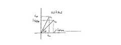
電動機トルクＴ_ｍに対して基準トルクＴ_ｒｅｆをプロットすると、理想的な適合例では原点で始まって勾配１を有する数式１のグラフを得ることができる。これを図１に示す。
【００２０】
回転子の時定数τ_２、τ_２＝τ’_２に対する回転子の推定時定数τ’_２がうまく適合していない場合には、関数Ｔ_ｒｅｆ＝ｆ（Ｔ_ｍ）の実際のプロファイルはこの線形特性とは異なるものとなる。図１にはこの関数の非適合時における基本特性も示してある。
【００２１】
図１から明らかなように、速度制御装置（τ’_２＜τ_２）における回転子の推定時定数τ’_２の値を小さくすると、速度制御装置（図示せず）によって算出される基準トルクＴ_ｒｅｆは過比例的に増加して与えられた電動機トルクＴ_ｍに達するが、昇降機系に加わるトルクＴ_ｍは簡単に測定パラメータとして得られるような類いのものではないため、適合を目的としてＴ_ｒｅｆ＝ｆ（Ｔ_ｍ）の関係を直接評価することは不可能である。しかしながら（インクリメンタルシャフトエンコーダによって）機械の速度ω_ｍを測定すれば求められる間接測定パラメータすなわち角加速度ω_ｍを利用することはできる。角加速度ω_ｍとトルクＴ_ｍとの関係は（摩擦を無視すれば）以下の数式２によって得られる。
【００２２】
【数２】
Ｔ_ｍ＝Ｊω_ｍ＋Ｔ_ＬＯＡＤ⇔ω_ｍ＝（Ｔ_ｍ−Ｔ_ＬＯＡＤ）／Ｊ
数式２によれば、角加速度ω_ｍはＴ_ｍに基づく線形のグラフとなる。従って、角加速度ω_ｍを機械のトルクＴ_ｍについての測定値として用いることができる。ここで、基準速度と実速度との間の誤差は小さいと仮定すると、ω_ｍの数字的に好ましくない微分値に近似値ω_ｍ≒ω_ｒｅｆを代入することができる。ここで、ω_ｒｅｆはＩＭの基準角加速度である。
【００２３】
さて、理想適合状態（τ’_２＝τ_２）から始めるとすると、（Ｔ_ｍ＝Ｔ_ｒｅｆ）となる。ω≒ω_ｒｅｆとＴ_ｒｅｆとの関係は、上述の数式２から以下の数式３によって得ることができる。
【００２４】
【数３】
Ｔ_ｒｅｆ＝Ｊω_ｒｅｆ＋Ｔ_ＬＯＡＤ
関数Ｔ_ｒｅｆ＝ｆ（ω_ｒｅｆ）のグラフは、勾配ＪでオフセットＴ_ＬＯＡＤの直線になる。理想適合状態τ’_２＝τ_２という仮定が成り立たない場合には、直線の勾配とオフセットが変わるだけであとは図１と同じことが言える。
【００２５】
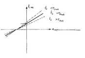
図２は、ＩＭのトルクについての測定値として使用するω_ｒｅｆと、速度制御装置における回転子の推定時定数τ’_２の理想値τ_２からの偏差についての基準トルクＴ_ｒｅｆとの基本的な関係を示す。
【００２６】
以下の説明では、Ｔ_ｒｅｆおよびω_ｒｅｆの代わりにＩ_Ｔｒｅｆおよびａ_ｒｅｆを制御系の内部パラメータとして用いる。換算基準加速度ａ_ｒｅｆは、定数の係数（ａ_ｒｅｆ＝ω_ｒｅｆ×ｒ_Ｔ／ｕ）以外は基準角加速度ω_ｒｅｆに対応する。同様に、トルク形成固定子電流成分Ｉ_ＴｒｅｆはＴ_ｒｅｆに正比例する。トルク電流基準値Ｉ_Ｔｒｅｆは、負荷トルクＴ_ＬＯＡＤに正比例する静的な部分Ｉ_{Ｔｓｔａｔ}と、加速度トルクＴ_{ＡＣＣＥＬＥＲＡＴＩＯＮ}または基準加速度ａ_ｒｅｆに正比例する動的な部分Ｉ_ＴＤＹＮとに分けることができる。Ｉ_Ｔｒｅｆとａ_ｒｅｆとの関係から、速度制御装置において機械の実際の回転子の時定数τ_２の値はどの程度推定値τ’_２と一致しているか分かる。判定基準を展開し、値Ｉ_Ｔｒｅｆおよびａ_ｒｅｆを評価することによってτ’_２のチューニング用の測定値を得る。本発明による適合方法の適用例の構造を図３に示す。
【００２７】
電流−加速度関係についての評価
以下の数式４に示す一次方程式によって適当な動作点の周囲（例えばａ_ｍａｘ／２付近など）において関数Ｉ_Ｔｒｅｆ＝ｆ（ａ_ｒｅｆ）を近似することができる。
【００２８】
【数４】
Ｉ_ｒｅｆ≒Ａａ_ｒｅｆ＋Ｂ ｗｉｔｈＢ−Ｔ_ＬＯＡＤ
ここで、係数Ａすなわち上述した直線の勾配は、選択した動作点を中心とした（小さな）変化についての基準加速度ａ_ｒｅｆと電流Ｉ_Ｔｒｅｆの基準値との間の増幅係数となる。オフセットＢは静負荷トルクＴ_ＬＯＡＤによって変化するが、τ_２＝τ’_２である場合に限ってＢはＴ_ＬＯＡＤに正比例する。従って、言うまでもなく「Ａ」は速度制御装置の回転子の時定数τ’_２のチューニングの関数となる。このチューニング用の測定値として、比ｖ＝τ_２／τ’_２を規定する。以下、数式５に示すような関係について定量的に検討する。
【００２９】
【数５】
Ａ＝Ｆ（ｖ）ただしｖ＝τ_２／τ’_２
Ｉ_Ｔｒｅｆおよびａ_ｒｅｆのプロファイルについての理論的研究
ａ_ｒｅｆとＩ_Ｔｒｅｆとの一般的な関係を系の動きについての式から得る。加速度トルクＴ_{ＡＣＣＥＬＥＲＡＴＩＯＮ}については以下の数式６が得られる。
【００３０】
【数６】

【００３１】
理想適合状態（τ’_２＝τ_２）の場合における誘導電動機（図４に示す等価回路）のトルクの適応部分は以下の数式７で示す値をとる。
【００３２】
【数７】

【００３３】
速度制御装置の理想的な動特性についての別の仮定のもとで、電流および加速度トルクについての実際の値に上述の式で得られた基準値を代入する。
【００３４】
数式６および７から、「動的」電流成分Ｉ_ＴＤＹＮ（数式４参照）について以下の数式８を得る。
【００３５】
【数８】

【００３６】
「静的」電流成分Ｉ_{Ｔｓｔａｔ}は、数式７における電流トルク関係からＩ_{Ｔｓｔａｔ}＝Ｔ_ＬＯＡＤ／（ｋＩ_ｆｌｕｘ）＝Ｂとして直接求めることができる。
【００３７】
全体として、τ’_２＝τ_２の場合には以下の数式９によって電流Ｉ_Ｔｒｅｆを算出することができる。
【００３８】
【数９】

【００３９】
係数Ａの分母ＫＩ_ｆｌｕｘもトルク−電流関係の微分増幅係数と解釈することができる。ここで、比適合状態（τ’_２≠τ_２）の場合を無視すると、ａ_ｒｅｆのプリファクターＡは一定ではなくなり、数式９は∂Ｔ_ｍ／∂Ｉ_Ｔｒｅｆ＝ｋＩ_ｆｌｕｘを用いて以下の数式１０のように表すことができる。
【００４０】
【数１０】

【００４１】
ＡＰは、電動機トルクＴ_ｍの偏導関数が求められる動作点である。動作点では「動的」電流成分Ｉ_ＴＤＹＮの平均値を用いることができる。従って、数式４から得られる係数Ａを以下の数式１１によって算出することができる。
【００４２】
【数１１】

【００４３】
回転子の時定数τ_２のチューニングによるＡへの影響を評価できるようにするために、トルクＴ_ｍに対する非適合状態による影響を考慮した一般化トルク−電流関係を導き出さなければならない。
【００４４】
一般化電流トルク式
まず、以下の数式１２に示す回転子−磁束関連座標における機械についての一般的なトルク式から説明する。
【００４５】
【数１２】

【００４６】
固定子電流ｉ_ｌについての滑り周波数ω_２と成分ｉ_１βおよびｉ_１αとの関係は以下の数式１３のようになる。
【００４７】
【数１３】

【００４８】
よって、トルクは以下の数式１４のように算出できる。
【００４９】
【数１４】

【００５０】
速度制御装置は以下の数式１５に基づいて機械の滑り周波数ω_２を特定した。
【００５１】
【数１５】

【００５２】
速度制御式機械のトルクは以下の数式１６のようになる。
【００５３】
【数１６】

【００５４】
電流ｉ_１αｓおよびｉ_１βｓの基準値や速度制御装置ｖ＝τ_２／τ’_２における回転子の時定数τ_２のチューニングの測定値からＴ_ｍのみを決定できるようにするために、上記数式１６における電流ｉ_１αにＩ_ＴｒｅｆおよびＩ_ｆｌｕｘを代入しなければならない。
【００５５】
図５に示すベクトル図および基本式ｔａｎφ＝ω_２τ_２からの固定子電流の基準値と実測値の大きさは等しいという仮定（「高速」電流制御および整流器）、さらにｔａｎφについての機械の滑り周波数に関する数式１５に基づいて、以下の数式１７を導き出すことができる。
【００５６】
【数１７】

【００５７】
また、図５から代入対象となる成分ｉ_１αについて以下の数式１８を得ることができる。
【００５８】
【数１８】

【００５９】
ここで、数式１９を代入し、さらにＩ_ｆｌｕｘについての数式１７から以下の数式２０を得ることができる。
【００６０】
【数１９】

【００６１】
【数２０】

【００６２】
従って、数式１６は以下の数式２１のように表すことができる。
【００６３】
【数２１】

【００６４】
数回にわたる変換によって、電流トルク関係を示す最終的な形を得ることができる。これを数式２２に示す。
【００６５】
【数２２】

【００６６】
ここで、速度制御装置が最適なレベルにあるとすれば、τ_２＝τ’_２であって数式２２はＴ_ｍ＝ｋＩ_ｆｌｕｘＩ_Ｔｒｅｆになる。
【００６７】
判定基準について
トルクＴ_ｍは測定量としては得られないので、回転子の推定時定数τ’_２のチューニングによるＴ_ｍ＝ｆ（Ｉ_Ｔｒｅｆ，τ_２／τ’_２）の特徴線の分枝の勾配への影響をそのまま系の適合状態についての判定基準として使用することはできない。しかしながら、数式１１を用いれば、制御系の内部パラメータとして得られる基準加速度ａ_ｒｅｆと基準電流値Ｉ_Ｔｒｅｆとの関係から上述の影響について間接的に評価することは可能である。係数Ａは勾配を示し、より正確にいうならば動作点ＡＰにおける関数Ｉ_Ｔｒｅｆ＝ｆ（ａ_ｒｅｆ）の増幅係数を示す。
【００６８】
偏導関数∂Ｔ_ｍ／∂Ｉ_Ｔｒｅｆの算出後、Ａについて以下の数式２３を得る。
【００６９】
【数２３】

【００７０】
理想的な適合状態τ’_２＝τ_２の場合について、数式８から得られるすでに分かっているＡについての式で数式２３をまとめると、Ａ＝Ｊｋ_ｖ／（ｋＩ_ｆｌｕｘ）＝一定が得られる。
【００７１】
Ｂ．適用
本発明を適用するための構成と共に計算式を少なくした本発明のより一層簡単な形について説明する。上述した形の方が高精度であるが、これは以下に述べる方法に比べて処理オーバーヘッドに対して費用をかけているがためである。
【００７２】
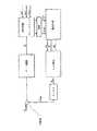
図６はベクトル制御式誘導電動機のブロック図である。速度制御装置は、速度基準値、加速度基準値、タコメータによって得られる誘導電動機の実速度、誘導電動機回転子の時定数に応答する。速度制御装置は、トルク電流基準値および磁束コマンドを独立に制御して出力することによって誘導電動機の速度を制御する。トルク電流基準値Ｉ_Ｔｒｅｆおよび磁束コマンドＩ_ｆｌｕｘは固定子電流の２つの成分である。これらの２つの成分は固定子電流調節器に供給される。固定子電流制御部は、固定子の三相電流のうちのＩ_ｕとＩ_ｖおよび回転子の実測角度Ｐｈｉに応答し、逆変換回路に固定子の三相電圧Ｕ_ｕ、Ｕ_ｖ、Ｕ_ｗを供給する。逆変換回路は固定子の三相電流に応答して誘導電動機にＵ_ｕ、Ｕ_ｖ、Ｕ_ｗを供給する。
【００７３】
理想的には、電動機トルクＴ_ｍとＴ_ｒｅｆとの関係は線形かつ１：１である。図１を参照のこと。実際には、このようなことは有り得ない。回転子の推定時定数τ’_２の値が変化し、これに対応する電動機トルクＴ_ｍおよびトルク基準値Ｔ_ｒｅｆの値を測定すればＴ_ｍ対Ｔ_ｒｅｆの直線は回転していることが分かる。従って、Ｔ_ｍ対Ｔ_ｒｅｆ直線の理想的な１：１関係からの変動量を決定することができれば、この変動量を回転子の理想時定数τ_２に対応して変化する回転子の推定時定数τ’_２と関連付けることができる。よって、実測Ｔ_ｍ対Ｔ_ｒｅｆ直線と１：１関係との間の変動量を利用して、Ｔ_ｍ対Ｔ_ｒｅｆ直線を１：１線形関係に戻すことのできる回転子の推定時定数τ’_２を生成することができる。
【００７４】
Ｔ_ｒｅｆ対Ｔ_ｍがどのように変化するか知るためにはＴ_ｍとＴ_ｒｅｆとを決めなければならない。Ｔ_ｒｅｆは決まっているので、残っているのはＴ_ｍだけである。従って、当然次のステップはＴ_ｍセンサを用いたＴ_ｍの算出になる。しかしながら、Ｔ_ｍセンサを使用せずにＴ_ｍを算出してコストを抑えることもできる。すなわち、より簡単かつ低費用で得られる値、基準加速度ａ_ｒｅｆおよび負荷トルクＴ_ＬＯＡＤに関する電動機トルクＴ_ｍを以下の数式２４から求めることができる。
【００７５】
【数２４】

【００７６】
このように、Ｔ_ｍとＴ_ｒｅｆがどのように変化するかはＴ_ｒｅｆとＡａ_ｒｅｆ＋Ｔ_ＬＯＡＤでどのように変化するかによって判断することができる。また、Ｔ_ｒｅｆはトルク電流基準値Ｉ_Ｔｒｅｆに正比例していることも分かる。簡単に言えば、Ｔ_ｍとＴ_ｒｅｆとの間の線形関係はＩ_ｒｅｆとａ_ｒｅｆ＋Ｔ_ＬＯＡＤの間の線形関係によって表すこともできるのである。電動機の速度が例えば０など一定であってトルク電流基準値Ｉ_Ｔｒｅｆに加速度トルク成分が含まれないような場合には、トルク電流基準値Ｉ_Ｔｒｅｆを測定することによってＴ_ＬＯＡＤを求めてもよい。加速度トルクが全くなければ、必要なトルクは負荷トルクＴ_ＬＯＡＤに対するものだけになるため、負荷トルクＴ_ＬＯＡＤはトルク電流基準値Ｉ_Ｔｒｅｆに正比例する。定速では加速度トルクＴ_{ＡＣＣＥＬＥＲＡＴＩＯＮ}は全く必要ない。従って、この直線勾配とオフセットの変化は、理想的な回転子の時定数τ_２からの回転子の推定時定数τ’_２の変化を示すものとなる。図７を参照のこと。
【００７７】
図７における直線は、直線Ｔ_ｍ対Ｔ_ｒｅｆの回転（図１）と全く同じように選択する回転子の推定時定数τ’_２によって回転する。図７におけるオフセットＢは、加速度がなく加速度トルクも全くない状態ではトルク電流基準値Ｉ_Ｔｒｅｆの値と等しい。このオフセットＢは、数式５において示すようにτ_２＝τ’_２である場合に限って負荷トルクＴ_ＬＯＡＤに正比例する。しかしながら、ＢはＴ_ＬＯＡＤと同一の符号を有する。ａ_ｒｅｆ＝０であってＴ_ｍ＝Ｔ_ＬＯＡＤである場合には数式２２および数式９を参照のこと。τ_２＝τ’_２であるとすると、Ｔ_ＬＯＡＤ＝ＫＩ_ｆｌｕｘ×Ｉ_Ｔｒｅｆになり、Ｉ_Ｔｒｅｆ＝Ｂになる。
【００７８】
図７における直線の勾配ＡをオフセットＢに対してプロットすると、図８および図９に示すグラフが得られる。この勾配Ａは数式４の勾配Ａと全く同じである。図８は、回転子の推定時定数τ’_２の様々な値についてのかごの上り方向への加速時または下り方向への減速時に得られる勾配Ａ対オフセットＢのグラフである。図９は、回転子の推定時定数τ’_２の様々な値についてのかごの下り方向への加速時または上り方向への減速時に得られる勾配Ａ対オフセットＢのグラフである。負荷トルクＴ_ＬＯＡＤが０より大きい図８において、回転子の推定時定数τ’_２と勾配Ａとの関係は特徴的なものとなる。図９において、負荷トルクＴ_ＬＯＡＤは０未満であり、回転子の推定時定数τ’_２と勾配Ａとの関係は特徴的なものとなる。よって、勾配ＡとオフセットＢとの関係は、負荷トルクＴ_ＬＯＡＤが０より大きい場合と負荷トルクＴ_ＬＯＡＤが０未満である場合について、それぞれ以下の数式２５および２６で表すことができる。
【００７９】
【数２５】

【００８０】
【数２６】

【００８１】
ここで、Ａ_１は上り方向への加速時または下り方向への減速時の図７に示す直線の勾配であり、Ａ_２は下り方向への加速時または上り方向への減速時の図７に示す直線の勾配；Ａ_０は回転子の推定時定数τ_２＝τ’_２である理想的な適合時の図７に示す直線の勾配；Ｃ_１およびＣ_２はそれぞれ図８および図９に示す直線の線形部分の勾配である。
【００８２】
Ｃ_１およびＣ_２は駆動系の慣性（回転慣性）に関連している。この慣性は上述の数式Ｔ_Ｍ＝Ａａ_ｒｅｆ＋Ｔ_ＬＯＡＤにおけるＡに関連している。すなわち、Ｔ＝Ｊ×ｄωｒ／ｄｔ＋Ｔ_ＬＯＡＤ（回転）である。ここでＪは電動機の駆動系の回転慣性である。この第２の式は上記の数式の一般例である。
【００８３】
ａ_ｒｅｆとｄωｒ／ｄｔとは等しくないためＡとＪとは等しくならない。誘導電動機の回転慣性に正比例するのでＣ_１およびＣ_２はほぼ等しいと考えることができる。
【００８４】
図６に示す直線Ｉ_Ｔｒｅｆ対ａ_ｒｅｆの勾配の同じ直線のオフセットに対するグラフは、上り方向への加速時または下り方向への減速時で負荷トルクが０より大きい場合および下り方向への加速時または上り方向への減速時で負荷トルクが０未満である時の勾配と回転子の推定時定数τ’_２との特徴的な関係を示す直線となる。従って、この勾配を判定基準として利用して回転子の推定時定数τ’_２が回転子の実時定数τ_２にうまく適合しているか否かを判定できる。勾配Ａ_０を理想勾配Ａ_０，_{ｉｄｅａｌ}から減算し、これによって得られる両者の差を比例積分回路に供給して回転子の推定時定数τ’_２を生成する。この回転子の推定時定数は、Ｔ_ｍ対Ｔ_ｒｅｆ直線を１：１線形関係に戻すことのできるものである。
【００８５】
図１０は本発明の適用例を示す図である。機能的に図６と同様の速度制御装置は、速度基準値、加速度基準値、電動機速度、回転子の推定時定数に応答して、磁束とトルクに関連する固定子電流の２つの成分を独立に制御する。速度制御装置は１０ミリ秒のクロックで動作して加速度基準値をサンプリングするとともに、これに対応するトルク電流基準値Ｉ_Ｔｒｅｆを算出する。この部分は本発明のなかで昇降機の動作時に実行しなければならない唯一の部分である。
【００８６】
サンプリングしたトルク電流基準値Ｉ_Ｔｒｅｆおよび加速度基準値ａ_ｒｅｆの値は、Ｉ_Ｔｒｅｆとａ_ｒｅｆとの線形関係の勾配ＡとオフセットＢを算出する線形回帰ブロックに供給されるまで格納される。Ａ_１は昇降機の上り方向への加速時または下り方向への減速時における勾配であり、Ａ_２は昇降機の下り方向への加速時または上り方向への減速時における勾配である。Ｂは加速と減速の両方について同一である。線形回帰ブロックは、Ｉ_Ｔｒｅｆ対ａ_ｒｅｆ直線の無負荷状態での勾配を算出するブロックにＡ_１、Ａ_２、Ｂを供給する。このブロックは、まず加速または減速の判定基準を使用すべきであるか否かを図８および図９に基づいて決定する。表２はＢの符号（＝負荷トルクＴ_ＬＯＡＤの符号）、昇降機の移動方向および加速度基準値とトルク電流基準値とのサンプル、加速相または減速相、使用する勾配の組み合わせを示す。
【００８７】
【表２】

続いてこのブロックは上記数式２５および２６からＡ_０を算出する。Ｃ_１およびＣ_２は、線形回帰ブロックや、Ａ_１、Ａ_２およびＢからＡ_０を算出するブロックでは得られない。Ｃ_１およびＣ_２は後述するような適用時において得られるものである。Ａ_０は次にノイズ抑制用のデジタルフィルタに供給される。この種のデジタルフィルタはＰｈｉｌｉｐｓ著『Ｄｉｇｉｔａｌ Ｃｏｎｔｒｏｌ ＳｙｓｔｅｍＡｎａｌｙｓｉｓ ａｎｄ Ｄｅｓｉｇｎ』第１２章に記載されている。次に、後述するような形で得られる回転子の時定数の実際の値に対応する理想値Ａ_０，_{ｉｄｅａｌ}からＩ_Ｔｒｅｆ対ａ_ｒｅｆの直線の実際の無負荷勾配Ａ_０を減算する。これによって得られた差を上述した文献の第８章に記載されているような比例積分制御装置に供給する。加算器からの差が負である場合には、回転子の推定時定数τ′_２は小さすぎるので比例積分制御装置から供給される回転子の推定時定数τ′_２の初期値を大きくするかまたはその逆にする。回転子の推定時定数τ′_２を増減することによって、Ｔ_ｍ対Ｔ_ｒｅｆを１：１に戻すことができ、図６に示すベクトル制御によって磁束とトルクとを独立して制御することができる。
【００８８】
本発明における初期化はＣ_１、Ｃ_２およびＡ_０，_{ｉｄｅａｌ}の決定にもからんでいる。
【００８９】
図１１は、Ａ_０を決定するための装置のブロック図である。まず、負荷トルクＴ_ＬＯＡＤをゼロに設定すなわちかご室の重量とかごの負荷を釣り合い重りと釣り合わせる。例えば誘導電動機用の識別アルゴリズムなどを利用して回転子の推定時定数τ′_２をτ_２の実際の値に設定する。この実際の値は例えばＨ．Ｓｃｈｉｅｒｌｉｎｇ著、Ｐｒｏｃ．ｏｆ Ｔｈｉｒｄ Ｉｎｔｅｒｎａｔｉｏｎａｌ Ｃｏｎｆｅｒｅｎｃｅ ｏｎ Ｐｏｗｅｒ Ｅｌｅｃｔｒｏｎｉｃｓ ａｎｄ Ｖａｒｉａｂｌｅ Ｓｐｅｅｄ Ｄｒｉｖｅ第２８７頁、『Ｓｅｌｆ−ｃｏｍｍｉｓｓｉｏｎｉｎｇ−−Ａ Ｎｏｖｅｌ Ｆｅａｔｕｒｅ ｏｆ Ｍｏｄｅｒｎ Ｉｎｖｅｒｔｅｒ−ｆｅｄ Ｉｎｄｕｃｔｉｏｎ Ｍｏｔｏｒ Ｄｒｉｖｅｓ』ＩＥＥＥ、Ｌｏｎｄｏｎ（１９８８年７月）などに記載されているような自己規定手順において得ることができる。かごを移動させ、トルク電流基準値Ｉ_Ｔｒｅｆと加速度基準値ａ_ｒｅｆとをサンプリングする。Ｂは０であるので、数式２５と２６の間には差はなく、Ａ_０，_{ｉｄｅａｌ}は線形回帰ブロックから供給される。
【００９０】
図１２は、回転子の推定時定数τ′_２の理想適合状態下にあるベクトル制御装置の理想値τ_２に対するブロック図である。ここで２つの初期化ランを取る、すなわち、空のかごを０未満の負荷トルクで上昇させてＣ_２を決め、空のかごを０より大きい負荷トルクで下降させてＣ_１を決定する。トルク電流基準値Ｉ_Ｔｒｅｆおよび加速度基準値ａ_ｒｅｆをサンプリングし、Ａ_０，_{ｉｄｅａｌ}と共にＡ_１、Ａ_２、Ｂを算出ブロックに供給し、Ｃ_１＝（Ａ_１−Ａ_０，_{ｉｄｅａｌ}）／Ｂ（負荷トルクＴ_ＬＯＡＤは０より大きい）およびＣ_２＝（Ａ_２−Ａ_０，_{ｉｄｅａｌ}）／Ｂ（負荷トルクＴ_ＬＯＡＤは０未満）を得る。
【００９１】
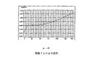
図１３は、回転子の推定時定数τ′_２および固定子温度を昇降機の動作回数に対してプロットした図である。回転子の時定数τ′_２は回転子の温度に正比例するため、この図は本発明が回転子の時定数を正しく推定していることを証明する良い例となる。固定子の温度は、定常状態では、回転子の温度と同じである。また、回転子の温度を変えるためには固定子の温度を回転子の温度の特性についての基準として用いることができる。
【００９２】
Ｓｃｈｉｅｒｌｉｎｇの誘導電動機の識別アルゴリズムに代わるアルゴリズムを以下に示す。
【００９３】
Ｃ．誘導機のパラメータ識別
１．機械モデル
この識別アルゴリズムは、Ｗ．Ｌｅｏｎｈａｒｄ著『Ｃｏｎｔｒｏｌ ｏｆ Ｅｌｅｃｔｒｉｃａｌ ｄｒｉｖｅｓ』、Ｓｐｒｉｎｇｅｒ−Ｖｅｒｌａｇ（Ｓｐｒｉｎｇｅｒ出版）、Ｂｅｒｌｉｎ， Ｈｅｉｄｅｌｂｅｒｇ， Ｎｅｗ Ｙｏｒｋ， Ｔｏｋｙｏ（１９８５年）に記載されているような周知の誘導電動機モデルとは若干異なる誘導電動機モデルに基づいている。以下の数式は本発明で使用するモデルを示すものである。これらの数式から、軸（ａ）および（ｂ）を有する座標系を使用した固定子固定座標における静止状態での誘導電動機がどのようなものか分かる。ここで、（ａ）は直線Ｒ、Ｓ、Ｔを有する三相電動機についての相のうちの１つの電動機相Ｒを示す。
【００９４】
【数２７】

【００９５】
【数２８】

【００９６】
このモデルは逆変換回路制御式昇降機の駆動制御装置を調節するために利用することもできる。数式２７および２８に示されるように、完全モデルを説明するために使用するパラメータは４つある。これらのパラメータは、固定子の抵抗Ｒ_１、回転子の時定数τ_２、全漏れインダクタンスＬ_σ、そして従来のモデルでは使われていないがこれら３つのパラメータから誘導できるパラメータＬ_Ｒである。Ｌ_Ｒ＝Ｌ_Ｈ^２／Ｒ^２であって、Ｌ_Ｈはメインインダクタンス、Ｒ_２は回転子の抵抗である。等価回路を図４に示す。
【００９７】
全漏れインダクタンスＬ_σについては、本発明の一部ではないがＨ．Ｓｃｈｉｅｒｌｉｎｇ著、博士論文１９８７第６１〜６５頁『Ｓｅｌｆ−Ｃｏｍｍｉｓｓｉｏｎｉｎｇ−−Ａ Ｎｏｖｅｌ Ｆｅａｔｕｒｅ ｏｆ Ｍｏｄｅｒｎ Ｉｎｖｅｒｔｅｒ−Ｆｅｄ Ｉｎｄｕｃｔｉｏｎ Ｍｏｔｏｒ Ｄｒｉｖｅｓ』、Ｓｉｅｍｅｎｓ ＡＧ（西ドイツ）およびＨ．Ｓｃｈｉｅｒｌｉｎｇ著『Ｓｅｌｂｓｔｅｉｎｓｔｅｌｌｅｎｄｅｓ ａｎｄ ｓｅｌｂｓｔａｎｐａｓｓｅｎｄｅｓ Ａｎｔｒｉｅｂｓｒｅｇｅｌｓｙｓｔｅｍ ｆｕｒ ｄｉｅ Ａｓｙｎｃｈｒｏｎｍａｓｃｈｉｎｅ ｍｉｔ Ｐｕｌｓｑｅｃｈｓｅｌｒｉｃｈｔｅｒ』（Ｔｅｃｈｎｉｃａｌ Ｕｎｉｖｅｒｓｉｔｙ ｏｆ Ｄａｒｍｓｔａｄｔ，西ドイツ）に記載されているアルゴリズムを利用して識別する。
【００９８】
２．全漏れインダクタンスＬσの識別
数式２７においてｉ_１ａ＝０およびΨ_２ａ^Ｂ＝０に設定すると、以下の数式２９が得られる。
【００９９】
【数２９】

【０１００】
これらの前提条件のもとで、電動機電圧と電流の偏差から全漏れインダクタンスを算出することができる。さて、低電圧域におけるパルス制御式逆変換回路の上述したような誤差をなくすために、＞１００Ｖの範囲の高電圧を電動機に印加しなければならないので実際の設定電圧は所望の値に対応する。電流は極めて急速に高くなるので測定時間は短く、Ψ_２ａ^Ｂ＝０はほぼ満たされる。もう１つの条件であるｉ_１ａ＝０を満たすために、電流のゼロ交点で測定を行う。
【０１０１】
この測定を実際に行い得るのは、図１４に示すように印加電圧とこの電圧によって生じる電動機電流の存在する時間内になる。
【０１０２】
時刻ｔ_０において、正の電圧がａ方向に電動機に印加される。時刻ｔ_１において電流は予め定められた限界値に達する。この限界値は電動機の定格電流によって変わるが、安全上の理由から０．５Ｉ_{ｒａｔｅｄ}までに制限されている。続いて電圧は０まで降下し、誘導機の電流は周波数変換器の中間コンデンサを介して放電される。コンデンサにおける電圧の上昇は吸収エネルギすなわち電動機の吸収エネルギＥ＝０．５ｉ^２Ｌおよびコンデンサの吸収エネルギＥ＝０．５（Ｕ＋ｄＵ）^２Ｃに基づいて算出することができる。
【０１０３】
無負荷状態について見ると、中間回路電圧Ｕ＝５４０Ｖであり、全漏れインダクタンスは、ここで用いた電動機におけるＣ＝１ｍＦで最大３０ｍＨになる。また、電圧上昇Ｕｄ＝２．７８Ｖ＝０．５％が得られる。これは十分許容できる値である。
【０１０４】
次に、時刻ｔ_２において、負の電圧Ｕ_ａが電動機に印加される。電流はもう１つの予め定められた負の限界値まで降下する。これによって電圧は再び０になり、インダクタは放電し、全漏れインダクタンスの識別は終了する。時刻ｔ_２とｔ_３の間に、電動機電流のゼロ交点が検出される。このゼロ交点近辺のある時間ｄｔについて電動機の電流を決定し、そこから全漏れインダクタンスＬ_σ＝Ｕ_２ｄｔ／ｄｉ_２を求める。
【０１０５】
本発明では残りのパラメータＲ_１、τ_２、Ｌ_Ｒを求めるための識別アルゴリズムについても説明する。このアルゴリズムは、電動機の固定子電圧および固定子電流が全て定常状態にある時に効を奏する。固定子の電流および電圧が定常値にあるということは、単に電流および電圧を印加してこれがなくなるまで遷移させるには十分であると思われるだけの時間待っているだけで簡単に確認することができる。
【０１０６】
３．残りのパラメータの識別
周波数変換器を用いることで大きさおよび方位に基づいて電圧フェーザ（ｐｈａｓｅｒ）を予め設定することができる。従って、周波数変換器に供給される定格電圧フェーザを適当に変化させることで識別に必要な周波数ωの出力周波数変換器ａｃ電圧Ｕ_１ａを達成することができる。しかしながら、周波数変換器内で発生する作用（最小起動時間、むだ時間）の影響で、実際に設定される出力電圧対所望の公称値の基本波に位相のシフトが起こる。低電圧では、この位相シフトはここで使用した周波数変換器については５〜１０°に達する。したがって、くどいようではあるが公称電圧を識別用の基準値として使用することは不可能である。
【０１０７】
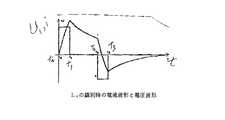
この問題に対する解決策の１つとして、電動機に図１５に示すように正弦電圧Ｕ_１ａではなく方形波を供給すればよい。
【０１０８】
図１５に示す矩形の固定子電圧Ｕ_１ａは電動機が静止状態にある時に供給する。電動機がトルクを発生せず止まったままでいるようにするために、もう１つの固定子電圧成分Ｕ_１ｂはゼロに設定しておく。固定子の電圧曲線は基本波ωと高調波とからなる。ωは時間Ｔ（図１参照）からω＝２π／Ｔによって導かれる。
【０１０９】
図１６は、図１５の固定子電圧ｕ_１ａから得られる電動機の固定子電流ｉ_１ａを示す。固定子電流ｉ_１ａの曲線はｕ_１ａの正負によって増減される指数関数からなる。
【０１１０】
図１７は、ｔａｎφを算出する本発明の一部を示す。角度φは電動機の固定子電圧の基本周波数と固定子電流との間の位相角を意味する。ｔａｎφは本発明のさらに他の部分で使用する。逆変換回路（３）は基本波ω_１（４）の所望の固定子電圧を誘導電動機（５）に供給する。固定子電圧は図１に示すものと同一である。Ａ／Ｄ変換器（７）を利用して時間Ｔで電動機の固定子電流（６）をサンプリングしてブロック（８）および（９）に供給する。ブロック（８）は、以下の数式３０に基づいて値ｙ_ｃを算出する。
【０１１１】
【数３０】

【０１１２】
数式３０において、ｉ_１ａ［ｋ］はｉ_１ａをサンプリングした値である。次にサンプリングされる値はｉ_１ａ［ｋ＋１］というふうになっていく。最初の値はｉ_１ａ［０］である。最後の値はｉ_１ａ［Ｔ／ｔ_{ｃｌｏｃｋ}−１］である。ブロック（８）の出力はｙ_ｃｏｓであり、ｙ_ｃの最終値に等しい。すなわち、以下の数式３１が得られる。
【０１１３】
【数３１】

【０１１４】
このように数式３０および数式３１は、時間的に連続した式の離散形態になっている。
【０１１５】
【数３２】

【０１１６】
ｉ_ｆｕｎｄ：ｉ_１ａ（ｔ）の基本周波数の振幅
数式３２は以下のようにして導き出される。
【０１１７】
ブロック（９）はブロック（８）での動作と同じようにして、数式３３、３４、３５に基づいてｙ_ｓｉｎ の値を算出する（数式３０、３１、３２参照）。
【０１１８】
【数３３】

【０１１９】
【数３４】

【０１２０】
【数３５】

【０１２１】
ブロック（１６）は除算を含む。このブロックは数式３６に基づいてｔａｎφを算出する。
【０１２２】
【数３６】

【０１２３】
図１８参照。全手順をｎ回実行する。ここで、ｎは図１において説明したような固定子の電圧曲線を電動機に供給する毎に得られるサンプルの数である。基本周波数ωの値は毎回変化する。従って、全繰り返しの結果は、基本周波数ωと適当なｔａｎφの値のｎ対からなる集合であり、以下の数式３７のように表すことができる。
【０１２４】
【数３７】

【０１２５】
本願明細書の以下の説明は、実測値Ｌ_σおよび数式３７を使用して残りの電動機のパラメータＲ_１、Ｌ_Ｒおよびτ_２を推定するアルゴリズムを示すものである。定常状態の場合には、電動機モデル（数式２７、２８）から数式３８のようにして固定子の複素インピーダンスＺ（ω）を導き出すことができる。
【０１２６】
【数３８】

【０１２７】
インピーダンスＺ（ω）の実成分および仮想成分は以下の数式３９で示すようになる。
【０１２８】
【数３９】

【０１２９】
さらに変換すると以下の数式４０のようになる。
【０１３０】
【数４０】

【０１３１】
インピーダンス量｜Ｚ（ω）｜の仮想部分はゼロである（この量は実数である）ので、以下の数式４１が得られる。
【０１３２】
【数４１】

【０１３３】
数式３８を数式４１に代入し、Ｒ（ω）およびＸ（ω）を数式２７および２８のパラメータに置き換えると、非線形式として以下の数式４２が得られる。
【０１３４】
【数４２】

【０１３５】
この数式４２は以下の数式４３〜５７に示すようにして得たものである。
【０１３６】
【数４３】

【０１３７】
【数４４】

【０１３８】
【数４５】

【０１３９】
【数４６】

【０１４０】
【数４７】

【０１４１】
【数４８】

【０１４２】
【数４９】

【０１４３】
【数５０】

【０１４４】
【数５１】

【０１４５】
【数５２】

【０１４６】
【数５３】

【０１４７】
【数５４】

【０１４８】
【数５５】

【０１４９】
【数５６】

【０１５０】
【数５７】

【０１５１】
この数式４７は数式３７のｎ動作点について書き替えることができる。書き替えによって得られる結果は以下の数式５８に示すようなｎ個の非線形式になる。
【０１５２】
【数５８】

【０１５３】
数式５８に示す式において、パラメータＬ_σ、ｔａｎφおよびωは分かっており、パラメータＲ_１、Ｌ_Ｒ、τ_２が抜けている。これらの足りないパラメータは数式４２を満たさなければならない。実際には、Ｌ_σおよびｔａｎφには測定誤差があるため数式４２に示す条件ｆ（Ｒ_１，Ｌ_Ｒ，τ_２）＝０を正確に満たすことは不可能である。
【０１５４】
また、ここでは測定による影響の他にも機械モデルの設定時の抜けなども原因となる。従って、足りないパラメータは数式４２を正確に満足させるのではなく近似させるのである。有効な近似値についての判定基準はｆ（Ｒ_１，Ｌ_Ｒ，τ_２）の二乗の最小化である（最小二乗法）。すなわち、以下の数式５９のようになる。
【０１５５】
【数５９】

【０１５６】
最小二乗法によって、１つ前のパラメータ集合（Ｒ_１，Ｌ_Ｒ，τ_２）［ｋ］から新しいパラメータ集合（Ｒ_１，Ｌ_Ｒ，τ_２）［ｋ＋１］を算出するための繰り返しパターンを構築することができる。推定した初期値（Ｒ_１，Ｌ_Ｒ，τ_２）［０］がＲ_１、Ｌ_Ｒ、τ_２を近似するのに適したものであれば、このアルゴリズムは足りないパラメータＲ_１，Ｌ_Ｒ，τ_２に収束する。
【０１５７】
これらのパラメータを図１８に示すように昇降機の電動機駆動装置に供給する。ベクトル制御用には、回転子の時定数を速度制御装置に供給する。
【０１５８】
上述した実施例には本発明の趣旨および範囲を逸脱することなく様々な修正を加えることができる。
【０１５９】
【発明の効果】
以上説明したように、本発明によれば、以下のような効果が得られる。
【０１６０】
（ａ）十分に適合したベクトル制御によって移動時間を短縮し、かつ快適な乗り心地を達成できる。
【０１６１】
（ｂ）固定子の電圧を測定せずに回転子の時定数を得ることができる。
【０１６２】
（ｃ）アルゴリズムを直線上で発揮でき、余計な移動時間の原因となる時間的な遅れはなくなる。
【０１６３】
（ｄ）Ｉ_Ｔｒｅｆおよびａ_ｒｅｆの算出に実行中にほんのわずかな計算時間を加えるだけでよく、殆どの計算は静止時に行うことができる。
【図面の簡単な説明】
【図１】Ｔ_ｒｅｆ対Ｔ_ｍのグラフである。
【図２】Ｔ_ｒｅｆ対ω_ｒｅｆ〜ωのグラフである。
【図３】本発明のブロック図である。
【図４】誘導電動機等価回路である。
【図５】Ｉ_Ｔｒｅｆ対Ｉ_ｆｌｕｘのグラフである。
【図６】ベクトル制御式誘導電動機のブロック図である。
【図７】Ｉ_Ｔｒｅｆ対ａ_ｒｅｆのグラフである。
【図８】Ａ対Ｂのグラフである。
【図９】Ａ対Ｂのグラフである。
【図１０】本発明を説明するためのブロック図である。
【図１１】初期化方法において使用する回路のブロック図である。
【図１２】初期化方法において使用する回路のブロック図である。
【図１３】回転子の推定時定数τ′_２および固定子温度（℃）対昇降機の数を示すグラフである。
【図１４】誘導電動機の全漏れインダクタンスＬ_σの識別に使用する固定子の電流および電圧波形を示すグラフである。
【図１５】回転子の時定数τ_２、回転子の抵抗Ｒ_１およびパラメータＬ_Ｒを識別するために使用する固定子の電圧を示すグラフである。
【図１６】回転子の時定数τ_２、回転子の抵抗Ｒ_１およびパラメータＬ_Ｒを識別するために使用する固定子の電流を示すグラフである。
【図１７】タンジェントφ対固定子周波数ωのグラフである。
【図１８】タンジェントφを得るための回路のブロック図である。[0001]
[Industrial application fields]
The present invention relates to a method for determining a time constant of a rotor used in a vector control induction motor.
[0002]
[Prior art]
Currently, many elevator drive units equipped with induction motors use vector control. When vector control is used, the dynamic characteristics of the motor are improved, and the elevator speed follows the reference value without any slight deviation, so the travel time can be shortened with a comfortable ride.
[0003]
In order to effectively use the advantages of this control method, it is necessary to know the electrical parameters of the motor to be controlled. In other words, the vector control means that the torque current is controlled completely independently of the magnetic flux control in the stator. Such independent control can be performed only when the time constant value of the rotor to be used is correct. K. B. Nordin, D.C. W. Novothy, D.C. S. See Zinger, The Inflation of Motor Parameter Development in Feedforward Field Orientation Drive Systems, IEEE IAS 84: 22B, page 525 (1984). Unfortunately, the rotor time constant is not constant and depends on the resistance of the rotor, which in turn depends on the rotor temperature, which varies with the load conditions of the elevator. There are many general algorithms for estimating the rotor time constant, but these algorithms either require extremely complex and expensive hardware, or use input and output values that are not available in elevator drives. Therefore, it is usually not suitable for a drive device for an elevator.
[0004]
[Problems to be solved by the invention]
There is also a kind of algorithm that supplies a specific noise signal to the motor and uses it. In this algorithm, the voltage, current and speed of the motor are measured, and the time constant of the rotor is calculated from these measurement results. However, if a noise signal is supplied to the electric motor, a sudden movement occurs and the ride comfort is deteriorated. Therefore, the noise signal cannot actually be supplied to the electric motor for the elevator and such an algorithm is not suitable for the elevator. R. Gabriel and W.W. See Leonhard, "Microprocessor Control of Induction Motor", IEEE (1982).
[0005]
Furthermore, there is an algorithm of a method for estimating a rotor time constant using a special operation mode such as idling or a specific speed, but such an operation mode cannot be used in an elevator. Proc. of the 18th Southwestern Symposium on System Theory, M.M. Song and J.M. See Mesca's "The the Identification of Induction Motor Parameters", IEEE, Knoxville, USA (April 1986).
[0006]
In addition, Proc. of Third International Conference on Power Electronics and Variable Speed Drive, p. 287, H.C. See Scherling, “Self Commissioning—A Novel Feature of Modern Inverter-Fed Induction Motor Drivers”, IEEE, London (July 1988). These documents deal with the determination of the rotor time constant using the stator voltage, but the problem here is that in elevators, the stator voltage is mostly measured for cost reasons. In other words, such an algorithm also becomes useless long.
[0007]
Therefore, the object of the present invention is to estimate the estimated time constant τ of the rotor of the vector controlled induction motor.₂Is adapted to the real time constant of the rotor.
[0008]
[Means and Actions for Solving the Problems]
The present invention firstly provides a torque reference value T for a vector controlled induction motor._refMotor torque T against_MThis graph is ideally a straight line with a gradient of 1, and secondly, the estimated time constant τ 'of the rotor supplied to the vector-controlled induction rotor.₂Note that the line rotates around the origin of the graph.
[0009]
The third point of focus in the present invention is T_MVs. T_refIf the fluctuation amount from the ideal 1: 1 linear relationship of the straight line can be obtained, this fluctuation amount is used as the real time constant τ of the rotor.₂Rotor estimated time constant τ '₂It is to be able to think in connection with. For this reason, T_MVs. T_refUsing the amount of variation from a 1: 1 linear relationship of straight lines, T_MVs. T_refEstimated rotor time constant τ 'capable of reproducing a linear 1: 1 linear relationship₂Ask for.
[0010]
T_MVs. T_refTo know how changes occur, T_MAnd T_refHave to ask. T_refIs decided, so what remains is T_MOnly. Therefore, naturally T_MT using sensor_MIs the next step. However, T_MT without using sensor_MThe cost can also be reduced by calculating. This is the fourth point of focus of the present invention. That is, a simpler and less expensive value, the reference acceleration a_refAnd load torque T_LOADMotor torque T_MThe formula T_M= Qa_ref+ T_LOADIt is to ask from. In this case, T_LOADCan only be obtained approximately, but the present invention requires a load torque T_LOADSince only the sign of is, an approximate value is sufficient. Therefore, T_MAnd T_refHow T changes_refAnd Qa_ref+ T_LOADCan be determined based on how the changes.
[0011]
Fifth, in the present invention, T_refIs the torque current reference value I_TrefWe also pay attention to the fact that it is directly proportional to.
[0012]
In short, T_MAnd T_refThe linear relationship between_refAnd a_ref+ T_LOADIt can also be expressed by a linear relationship between. Motor speed ω_mIs constant, for example 0, and I_TrefWhen the acceleration torque component is not included in the torque current reference value I_TrefBy measuring T_LOADYou may ask for. T if there is no acceleration torque_LOADIs I_TrefThis is because it is directly proportional to. Therefore, this straight line I_TrefVs. a_refThe change in slope and offset from the 1: 1 relationship of₂Estimated rotor time constant τ ′ from₂Changes.
[0013]
The sixth focus point of the present invention is the straight line I._refAnd a_refOffset (a_refIs 0 and acceleration torque T_ACCELERATIONThis offset is T_LOAD, And the estimated time constant τ 'of the rotor.₂It can be proved the linear relationship between T_LOADA characteristic linear relationship is obtained when> 0 and the elevator is accelerating in the upward direction or decelerating in the downward direction. T_LOADAnother characteristic linear relationship is obtained when <0 and the elevator is accelerating downward or decelerating upward. For this reason I_TrefVs. a_refThe estimated time constant τ ′ of the rotor using the gradient of₂Is the real time constant of the rotor τ₂It is possible to determine whether or not it fits well. In the no-load state, this gradient is subtracted from the ideal gradient, and the difference between the two is supplied to the proportional integration circuit to estimate the rotor time constant τ '.₂Is generated. The estimated time constant of this rotor is T_MVs. T_refThe straight line can be returned to the 1: 1 linear relationship which is very important in a vector controlled motor.
[0014]
According to the present invention, the torque current reference value I in the drive device for the vector controlled induction motor is provided._TrefAnd reference acceleration a_refIs extracted and the criterion is developed, whereby the estimated time constant τ ′ of the rotor₂The rotor real time constant τ₂To fit.
[0015]
More specifically, the torque current reference value I_TrefAnd reference acceleration a_refAfter sampling I_TrefVs. a_refThe gradient of the load torque T_LOADIs plotted against the offset of the straight line that is directly proportional to. From this plot, find the no-load gradient and subtract it from the ideal no-load gradient.₂Rotor estimated time constant τ ′₂Get.
[0016]
【Example】
In Table 1 below, subscript 1 indicates the stator value andsubscript 2 indicates the rotor value.
[0017]
[Table 1]
a_ref        Acceleration reference value
IM induction motor
V = τ₂/ Τ '₂
u Reduction ratio of elevator drive unit
r_T          Pulley radius of elevator drive
P 2P is the number of poles of the induction motor
J Rotational inertia of drive unit
kv u / r_T
k P³L_H²/ 2L₂
Z (ω) Stator complex inductance
T Stator current period
X (ω) Virtual part of stator impedance
φ Angle between stator current and voltage
I_Tref      Torque current reference value
i_flux      Magnetic flux current reference value
I_1α        Stator current component synchronized to rotating coordinates
i_1β        Stator current component synchronized to rotating coordinates
i_1a        Stator current
i_1b        Stator current
i_TSTAT      Static current component of torque current
i_TDYN      Dynamic current component of torque current
L_H          Induction motor equivalent circuit inductance
L₁          Stator inductance
L₂          Rotor inductance
L_σ          Total leakage inductance
L_1σ        Stator leakage inductance
L_2σ        Rotor leakage inductance
L_R          Main inductance
R (ω) Real part of stator impedance
R₁          Stator resistance
R₂          Rotor resistance
T_m          Motor torque
T_ref        Torque reference value
T_LOAD      Load torque
U_1a        Stator voltage
U_1b        Stator voltage
ω_m          Induction of motor speed
ω_m          Motor speed (rotation)
ω_ref        Reference motor speed
ω₁          Stator frequency
ω fundamental frequency of stator voltage
ω₂          Slip frequency
Ψ_2b        Stator magnetic flux
Ψ_2b        Stator magnetic flux
Ψ_2α        Rotor magnetic flux
τ₂          Real time constant of the rotor
τ ′₂        Estimated time constant of the rotor
A. General principle
Assuming that the vector control parameters for IM are set to ideal values and a high performance dynamic premium servo mechanism is used, the motor torque T_mIs the reference torque T required for vector control_refAlways matches. Therefore, the following formula 1 is obtained in an ideal example.
[0018]
[Expression 1]
T_m= T_ref
In addition to arbitrarily setting a current control loop that minimizes the control error rate for this ideal characteristic, the rotor time constant τ₂The basic precondition is that the current value of can be known accurately.
[0019]
Electric motor torque T_mWith reference torque T_ref, The ideal fit can be obtained as a graph of Equation 1 starting at the origin and having a slope of 1. This is shown in FIG.
[0020]
Rotor time constant τ₂, Τ₂= Τ ’₂Estimated rotor time constant τ ′ for₂Is not well suited, the function T_ref= F (T_m) Is different from this linear characteristic. FIG. 1 also shows the basic characteristics of this function when it is not compatible.
[0021]
As is apparent from FIG. 1, the speed control device (τ ′₂<Τ₂) Estimated rotor time constant τ '₂When the value of is reduced, the reference torque T calculated by the speed control device (not shown)_refIs an over-proportional increase in motor torque T_mTorque T applied to the elevator system_mIs not the kind that can be easily obtained as a measurement parameter._ref= F (T_m) Cannot be directly evaluated. However (by the incremental shaft encoder) the machine speed ω_mIndirect measurement parameters that can be obtained by measuring_mCan be used. Angular acceleration ω_mAnd torque T_m(If the friction is ignored),
[0022]
[Expression 2]
T_m= Jω_m+ T_LOAD⇔ω_m= (T_m-T_LOAD/ J
According toEquation 2, the angular acceleration ω_mIs T_mA linear graph based on Therefore, the angular acceleration ω_mThe machine torque T_mIt can be used as a measured value for. Here, assuming that the error between the reference speed and the actual speed is small, ω_mThe approximate value ω_m≒ ω_refCan be substituted. Where ω_refIs the reference angular acceleration of IM.
[0023]
Now, the ideal fit state (τ ′₂= Τ₂) Starts with (T_m= T_ref) ω ≒ ω_refAnd T_refThe following relationship can be obtained fromEquation 2 described above and Equation 3 below.
[0024]
[Equation 3]
T_ref= Jω_ref+ T_LOAD
Function T_ref= F (ω_ref) Is an offset T with a slope J_LOADIt becomes a straight line. Ideal fit state τ ’₂= Τ₂If this assumption does not hold, the same can be said as in FIG. 1 except that the slope and offset of the straight line change.
[0025]
Figure 2 shows the ω used as a measurement for IM torque_refAnd an estimated time constant τ ′ of the rotor in the speed control device₂Ideal value of τ₂Reference torque T for deviation from_refThe basic relationship is shown.
[0026]
In the following description, T_refAnd ω_refInstead of I_TrefAnd a_refIs used as an internal parameter of the control system. Conversion standard acceleration a_refIs a constant coefficient (a_ref= Ω_refXr_T/ U) is the reference angular acceleration ω_refCorresponding to Similarly, the torque forming stator current component I_TrefIs T_refIs directly proportional to Torque current reference value I_TrefIs the load torque T_LOADStatic part I directly proportional to_TstatAnd acceleration torque T_ACCELERATIONOr reference acceleration a_refDynamic part I directly proportional to_TDYNAnd can be divided into I_TrefAnd a_refThe time constant τ of the actual rotor of the machine in the speed control device₂Is the estimated value τ ’₂You can see if it matches. Develop criteria and value I_TrefAnd a_refBy evaluating τ ′₂Get measured values for tuning. The structure of an application example of the adaptation method according to the present invention is shown in FIG.
[0027]
Evaluation of current-acceleration relationship
Around the appropriate operating point (for example, a_maxIn the vicinity of / 2, etc.)_Tref= F (a_ref) Can be approximated.
[0028]
[Expression 4]
I_ref≒ Aa_ref+ B withB-T_LOAD
Here, the coefficient A, that is, the gradient of the straight line described above, is a reference acceleration a for a (small) change around the selected operating point._refAnd current I_TrefIt becomes an amplification coefficient between the reference values. Offset B is static load torque T_LOADDepends on τ₂= Τ ’₂B is T only if_LOADIs directly proportional to Therefore, needless to say, “A” is the time constant τ ′ of the rotor of the speed controller.₂It becomes a function of tuning. As a measured value for this tuning, the ratio v = τ₂/ Τ ’₂Is specified. Hereinafter, the relationship as shown in Formula 5 will be examined quantitatively.
[0029]
[Equation 5]
A = F (v) where v = τ₂/ Τ ’₂
I_TrefAnd a_refTheoretical study on profiles
a_refAnd I_TrefIs obtained from the equation for the movement of the system. Acceleration torque T_ACCELERATIONThe following equation 6 is obtained.
[0030]
[Formula 6]

[0031]
Ideal fit state (τ ’₂= Τ₂), The torque adaptive portion of the induction motor (equivalent circuit shown in FIG. 4) takes a value represented by the following Equation 7.
[0032]
[Expression 7]

[0033]
Under another assumption about the ideal dynamic characteristics of the speed controller, the reference value obtained from the above formula is substituted into the actual values for the current and acceleration torque.
[0034]
From Equations 6 and 7, the “dynamic” current component I_TDYNThe followingformula 8 is obtained for (see formula 4).
[0035]
[Equation 8]

[0036]
"Static" current component I_TstatFrom the current torque relationship in Equation 7_Tstat= T_LOAD/ (KI_flux) = B.
[0037]
Overall, τ ’₂= Τ₂In the case of the current I_TrefCan be calculated.
[0038]
[Equation 9]

[0039]
Denominator KI of coefficient A_fluxCan also be interpreted as a differential amplification coefficient of torque-current relationship. Here, the ratio matching state (τ ′₂≠ τ₂) Is ignored, a_refThe prefactor A is no longer constant and Equation 9 is ∂T_m/ ∂I_Tref= KI_fluxCan be expressed as inEquation 10 below.
[0040]
[Expression 10]

[0041]
AP is the motor torque T_mThis is the operating point at which the partial derivative of is obtained. At the operating point, the “dynamic” current component I_TDYNThe average value of can be used. Therefore, the coefficient A obtained fromEquation 4 can be calculated by Equation 11 below.
[0042]
[Expression 11]

[0043]
Rotor time constant τ₂In order to be able to evaluate the influence on A by tuning the torque, torque T_mA generalized torque-current relationship should be derived that takes into account the effects of non-conformance on
[0044]
Generalized current torque type
First, a general torque equation for the machine in the rotor-magnetic flux related coordinates shown in Equation 12 below will be described.
[0045]
[Expression 12]

[0046]
Stator current i_lAbout slip frequency ω₂And ingredient i_1βAnd i_1αThe relationship is as shown in Equation 13 below.
[0047]
[Formula 13]

[0048]
Therefore, the torque can be calculated as in the following Expression 14.
[0049]
[Expression 14]

[0050]
The speed control device calculates the machine slip frequency ω based on Equation 15 below.₂Identified.
[0051]
[Expression 15]

[0052]
The torque of the speed control type machine is as shown in the following Expression 16.
[0053]
[Expression 16]

[0054]
Current i_1αsAnd i_1βsReference value and speed control device v = τ₂/ Τ ’₂Rotor time constant τ₂T from the measured value of tuning_mTo determine only the current i in equation 16 above._1αI_TrefAnd I_fluxMust be assigned.
[0055]
The vector diagram shown in FIG. 5 and the basic expression tanφ = ω₂τ₂Based on the assumption that the magnitude of the reference and measured values of the stator current from (equal to “fast” current control and rectifier) is equal, and further to Equation 15 for machine slip frequency for tan φ, the following Equation 17 is derived: Can do.
[0056]
[Expression 17]

[0057]
Also, from FIG. 5, the component i to be substituted_1αThe following formula 18 can be obtained.
[0058]
[Formula 18]

[0059]
Here, Equation 19 is substituted, and further I_fluxThe followingformula 20 can be obtained from the formula 17 for.
[0060]
[Equation 19]

[0061]
[Expression 20]

[0062]
Therefore, Expression 16 can be expressed as Expression 21 below.
[0063]
[Expression 21]

[0064]
Several rounds of conversion can yield the final shape showing the current torque relationship. This is shown in Equation 22.
[0065]
[Expression 22]

[0066]
Here, if the speed control device is at an optimum level, τ₂= Τ ’₂And Equation 22 is T_m= KI_fluxI_Trefbecome.
[0067]
About judgment criteria
Torque T_mCannot be obtained as a measured quantity, so the estimated time constant τ '₂T by tuning_m= F (I_Tref, Τ₂/ Τ ’₂) On the gradient of the branch of the feature line cannot be used as a criterion for the compatibility of the system as it is. However, using Equation 11, the reference acceleration a obtained as an internal parameter of the control system_refAnd reference current value I_TrefIt is possible to indirectly evaluate the above-mentioned influence from the relationship. The factor A indicates the slope, more precisely the function I at the operating point AP._Tref= F (a_ref) Amplification factor.
[0068]
Partial derivative ∂T_m/ ∂I_TrefAfter calculating A, the following Expression 23 is obtained for A.
[0069]
[Expression 23]

[0070]
Ideal fit state τ ’₂= Τ₂In the case of the above, when the equation 23 is put together with the already known equation A obtained from theequation 8, A = Jk_v/ (KI_flux) = Constant is obtained.
[0071]
B. Application
A simpler form of the present invention in which the number of calculation formulas is reduced together with the configuration for applying the present invention will be described. The form described above is more accurate because it costs more processing overhead than the method described below.
[0072]
FIG. 6 is a block diagram of a vector control induction motor. The speed control device responds to the speed reference value, the acceleration reference value, the actual speed of the induction motor obtained by the tachometer, and the time constant of the induction motor rotor. The speed control device controls the speed of the induction motor by independently controlling and outputting the torque current reference value and the magnetic flux command. Torque current reference value I_TrefAnd magnetic flux command I_fluxAre two components of the stator current. These two components are fed to the stator current regulator. The stator current control unit is an I of the three-phase current of the stator._uAnd I_vAnd the three-phase voltage U of the stator in the inverter circuit in response to the measured angle Phi of the rotor._u, U_v, U_wSupply. The reverse conversion circuit responds to the three-phase current of the stator to the induction motor._u, U_v, U_wSupply.
[0073]
Ideally, the motor torque T_mAnd T_refIs linear and 1: 1. See FIG. In fact, this is not possible. Estimated time constant of rotor τ '₂Of the motor torque T corresponding to this change_mAnd torque reference value T_refIf you measure the value of T_mVs. T_refIt can be seen that the straight line is rotating. Therefore, T_mVs. T_refIf the amount of variation from the ideal 1: 1 relationship of the straight line can be determined, this amount of variation is converted to the ideal time constant τ of the rotor.₂Estimated time constant τ 'of the rotor that changes corresponding to₂Can be associated with Therefore, measured T_mVs. T_refUsing the amount of variation between the straight line and the 1: 1 relationship, T_mVs. T_refEstimated time constant τ 'of the rotor that can return the straight line to a 1: 1 linear relationship₂Can be generated.
[0074]
T_refVs. T_mTo see how changes occur_mAnd T_refYou must decide. T_refIs decided, so what remains is T_mOnly. Therefore, naturally the next step is T_mT using sensor_mIt becomes calculation of. However, T_mT without using sensor_mThe cost can also be reduced by calculating. That is, a simpler and less expensive value, the reference acceleration a_refAnd load torque T_LOADMotor torque T_mCan be obtained from Equation 24 below.
[0075]
[Expression 24]

[0076]
Thus, T_mAnd T_refHow T changes_refAnd Aa_ref+ T_LOADIt can be judged by how it changes. T_refIs the torque current reference value I_TrefIt can also be seen that it is directly proportional to. Simply put, T_mAnd T_refThe linear relationship between_refAnd a_ref+ T_LOADIt can also be expressed by a linear relationship between. The speed of the motor is constant, for example 0, and the torque current reference value I_TrefWhen the acceleration torque component is not included in the torque current reference value I_TrefBy measuring T_LOADYou may ask for. If there is no acceleration torque, the required torque is the load torque T_LOADLoad torque T_LOADIs the torque current reference value I_TrefIs directly proportional to At constant speed, acceleration torque T_ACCELERATIONIs not necessary at all. Therefore, the change in linear slope and offset is the ideal rotor time constant τ₂Estimated rotor time constant τ ′ from₂Changes. See FIG.
[0077]
The straight line in FIG._mVs. T_refEstimated rotor time constant τ 'selected in exactly the same way as the rotation of the rotor₂Rotate by. The offset B in FIG. 7 is a torque current reference value I in a state where there is no acceleration and no acceleration torque._TrefIs equal to the value of This offset B is expressed as τ as shown in Equation 5.₂= Τ ’₂Only when the load torque T_LOADIs directly proportional to However, B is T_LOADHave the same sign. a_ref= 0 and T_m= T_LOADIf so, see Equation 22 and Equation 9. τ₂= Τ ’₂If T_LOAD= KI_flux× I_TrefI_Tref= B.
[0078]
If the slope A of the straight line in FIG. 7 is plotted against the offset B, the graphs shown in FIGS. 8 and 9 are obtained. This gradient A is exactly the same as the gradient A inEquation 4. FIG. 8 shows the estimated rotor time constant τ ′.₂Is a graph of slope A versus offset B obtained when the car is accelerated in the upward direction or decelerated in the downward direction for various values of. FIG. 9 shows the estimated rotor time constant τ ′.₂Is a graph of slope A versus offset B obtained when the car is accelerating in the downward direction or decelerating in the upward direction.Load torque T_LOAD8 is greater than 0, the estimated rotor time constant τ '₂And the gradient A are characteristic. In FIG. 9, the load torque T_LOADIs less than 0 and the estimated rotor time constant τ '₂And the gradient A are characteristic. Therefore, the relationship between the gradient A and the offset B is the load torque T_LOADIs greater than 0 and the load torque T_LOADCan be represented by the following formulas 25 and 26, respectively.
[0079]
[Expression 25]

[0080]
[Equation 26]

[0081]
Where A₁Is the slope of the straight line shown in FIG. 7 during acceleration in the upward direction or deceleration in the downward direction.₂Is the slope of the straight line shown in FIG. 7 when accelerating downward or decelerating upward; A₀Is the estimated rotor time constant τ₂= Τ ’₂The slope of the straight line shown in FIG.₁And C₂Is the slope of the linear portion of the straight line shown in FIGS. 8 and 9, respectively.
[0082]
C₁And C₂Is related to the inertia of the drive train (rotational inertia). This inertia is expressed by the above formula T_M= Aa_ref+ T_LOADIs related to A. That is, T = J × dωr / dt + T_LOAD(Rotation). Here, J is the rotational inertia of the drive system of the electric motor. This second formula is a general example of the above formula.
[0083]
a_refAnd dωr / dt are not equal, so A and J are not equal. C is directly proportional to the rotational inertia of the induction motor.₁And C₂Can be considered almost equal.
[0084]
Straight line I shown in FIG._TrefVs. a_refThe graph for the offset of the straight line with the same slope of Gradient when less than 0 and estimated rotor time constant τ '₂It becomes a straight line showing a characteristic relationship with. Therefore, using this gradient as a criterion, the estimated time constant τ ′ of the rotor₂Is the real time constant of the rotor τ₂It is possible to determine whether or not it fits well. Gradient A₀The ideal gradient A₀,_idealAnd the difference between the two is supplied to the proportional integration circuit to estimate the rotor time constant τ '.₂Is generated. The estimated time constant of this rotor is T_mVs. T_refA straight line can be returned to a 1: 1 linear relationship.
[0085]
FIG. 10 is a diagram showing an application example of the present invention. The speed controller functionally similar to FIG. 6 is independent of the two components of the stator current associated with magnetic flux and torque in response to the speed reference value, acceleration reference value, motor speed, and estimated rotor time constant. To control. The speed control device operates with a 10 millisecond clock to sample the acceleration reference value and the corresponding torque current reference value I._TrefIs calculated. This is the only part of the present invention that must be performed during elevator operation.
[0086]
Sampled torque current reference value I_TrefAnd acceleration reference value a_refThe value of is I_TrefAnd a_refAre stored until they are supplied to the linear regression block for calculating the gradient A and the offset B of the linear relationship. A₁Is the gradient when the elevator is accelerated in the upward direction or decelerated in the downward direction.₂Is the gradient when the elevator is accelerating in the downward direction or decelerating in the upward direction. B is the same for both acceleration and deceleration. The linear regression block is I_TrefVs. a_refA block for calculating the slope of a straight line with no load₁, A₂, B is supplied. This block first determines based on FIGS. 8 and 9 whether acceleration or deceleration criteria should be used. Table 2 shows the sign of B (= load torque T_LOAD), A moving direction of the elevator, a sample of an acceleration reference value and a torque current reference value, an acceleration phase or a deceleration phase, and a combination of gradients to be used.
[0087]
[Table 2]

Subsequently, this block is obtained from the above equations 25 and 26 as A₀Is calculated. C₁And C₂Is a linear regression block or A₁, A₂And B to A₀It cannot be obtained from the block that calculates. C₁And C₂Is obtained at the time of application as described later. A₀Is then supplied to a digital filter for noise suppression. This type of digital filter is described in chapter 12 of Philips, Digital Control System Analysis and Design. Next, an ideal value A corresponding to the actual value of the time constant of the rotor obtained in the form described later.₀,_idealTo I_TrefVs. a_refActual no-load gradient A₀Is subtracted. The difference thus obtained is supplied to a proportional-integral controller as described inChapter 8 of the above-mentioned document. If the difference from the adder is negative, the estimated rotor time constant τ ′₂Is too small, so the estimated time constant τ ′ of the rotor supplied from the proportional integral controller₂Increase the initial value of or vice versa. Estimated time constant of rotor τ ′₂By increasing or decreasing_mVs. T_refCan be returned to 1: 1, and the magnetic flux and torque can be controlled independently by the vector control shown in FIG.
[0088]
The initialization in the present invention is C₁, C₂And A₀,_idealAlso involved in the decision.
[0089]
FIG.₀FIG. 2 is a block diagram of an apparatus for determining First, load torque T_LOADIs set to zero, that is, the weight of the cab and the load of the car are balanced with the balance weight. For example, an estimated time constant τ ′ of the rotor using an identification algorithm for an induction motor₂Τ₂Set to the actual value of. This actual value is for example H.264. Schierling, Proc. of Third International Conference on Power Electronics and Variable Speed Drive, etc. Can be obtained in a self-defining procedure. Move the car and the torque current reference value I_TrefAnd acceleration reference value a_refAnd sampling. Since B is 0, there is no difference between Equations 25 and 26 and A₀,_idealIs supplied from a linear regression block.
[0090]
FIG. 12 shows the estimated time constant τ ′ of the rotor₂The ideal value τ of the vector controller under ideal ideal condition₂FIG. Now take two initialization runs, i.e. raise the empty car with a load torque less than 0 and₂And lower the empty car with a load torque greater than 0 to₁To decide. Torque current reference value I_TrefAnd acceleration reference value a_refIs sampled and A₀,_idealWith A₁, A₂, B to the calculation block and C₁= (A₁-A₀,_ideal) / B (Load torque T_LOADIs greater than 0) and C₂= (A₂-A₀,_ideal) / B (Load torque T_LOADIs less than 0).
[0091]
FIG. 13 shows the estimated time constant τ ′ of the rotor₂It is the figure which plotted the stator temperature with respect to the frequency | count of operation | movement of an elevator. Rotor time constant τ ′₂Since is directly proportional to the rotor temperature, this figure is a good example to prove that the present invention correctly estimates the rotor time constant. The stator temperature is the same as the rotor temperature in the steady state. In order to change the temperature of the rotor, the temperature of the stator can be used as a reference for the temperature characteristics of the rotor.
[0092]
An algorithm that replaces the Scherling induction motor identification algorithm is shown below.
[0093]
C. Induction machine parameter identification
1. Machine model
This identification algorithm is described in W.W. Well known induction motor models such as those described in Leonhard's “Control of Electrical drives”, Springer-Verlag (published by Springer), Berlin, Heidelberg, New York, Tokyo (1985). ing. The following formula shows the model used in the present invention. From these equations, it can be seen what the induction motor is stationary in the stator fixed coordinates using a coordinate system with axes (a) and (b). Here, (a) shows one motor phase R of the phases for a three-phase motor having straight lines R, S, T.
[0094]
[Expression 27]

[0095]
[Expression 28]

[0096]
This model can also be used to adjust the drive control system of an inverse conversion circuit controlled elevator. As shown inequations 27 and 28, there are four parameters used to describe the complete model. These parameters are the stator resistance R₁, Rotor time constant τ₂, Total leakage inductance L_σAnd a parameter L that is not used in the conventional model but can be derived from these three parameters._RIt is. L_R= L_H²/ R²And L_HIs the main inductance, R₂Is the resistance of the rotor. An equivalent circuit is shown in FIG.
[0097]
Total leakage inductance L_σIs not part of the present invention, but H. Schering, Ph.D. 1987, pages 61-65, “Self-Commissioning—A Novel Feature of Modern Inverter-Fed Induction Motor Drives”, Siemens AG (West Germany) and H.C. Identified by Scherling's “Selbsteinstellendes and selbstanpassends Antriebregregsystem system fur die asynchronaschin mit Pulchschelrichter” (Technical Unit).
[0098]
2. Identification of total leakage inductance Lσ
InFormula 27, i_1a= 0 and Ψ_2a^BWhen = 0, the following formula 29 is obtained.
[0099]
[Expression 29]

[0100]
Under these preconditions, the total leakage inductance can be calculated from the deviation between the motor voltage and current. Now, in order to eliminate the above-described error of the pulse-controlled inverse conversion circuit in the low voltage range, a high voltage in the range of> 100 V must be applied to the motor, so the actual set voltage corresponds to the desired value. . Since the current increases very rapidly, the measurement time is short and Ψ_2a^B= 0 is almost satisfied. Another condition is i_1aTo satisfy = 0, the measurement is performed at the zero crossing point of the current.
[0101]
This measurement can actually be performed within the time when the applied voltage and the motor current generated by this voltage exist as shown in FIG.
[0102]
Time t₀, A positive voltage is applied to the motor in the direction a. Time t₁The current reaches a predetermined limit value at. This limit value depends on the rated current of the motor, but is 0.5I for safety reasons._ratedLimited to. Subsequently, the voltage drops to 0 and the induction machine current is discharged through the intermediate capacitor of the frequency converter. The rise in voltage at the capacitor is caused by the absorbed energy, that is, the absorbed energy E of the motor E = 0.5i.²L and absorbed energy of capacitor E = 0.5 (U + dU)²C can be calculated based on C.
[0103]
Looking at the no-load state, the intermediate circuit voltage U is 540 V, and the total leakage inductance is 30 mH at maximum at C = 1 mF in the motor used here. Further, a voltage increase Ud = 2.78 V = 0.5% is obtained. This is a sufficiently acceptable value.
[0104]
Next, time t₂Negative voltage U_aIs applied to the motor. The current drops to another predetermined negative limit value. As a result, the voltage becomes zero again, the inductor is discharged, and the identification of the total leakage inductance is completed. Time t₂And t₃During this time, the zero crossing point of the motor current is detected. The current of the motor is determined for a certain time dt in the vicinity of the zero crossing point, and the total leakage inductance L is determined therefrom._σ= U₂dt / di₂Ask for.
[0105]
In the present invention, the remaining parameter R₁, Τ₂, L_RAn identification algorithm for obtaining the above will also be described. This algorithm is effective when the stator voltage and stator current of the motor are all in a steady state. The fact that the stator current and voltage are at a steady value can be easily confirmed by simply waiting for the time that seems to be sufficient to apply the current and voltage and make the transition until it disappears. it can.
[0106]
3. Identify remaining parameters
By using the frequency converter, the voltage phasor can be preset based on the size and orientation. Accordingly, by appropriately changing the rated voltage phasor supplied to the frequency converter, the output frequency converter ac voltage U of the frequency ω necessary for identification is obtained._1aCan be achieved. However, due to the effects (minimum start-up time, dead time) occurring in the frequency converter, a phase shift occurs between the actually set output voltage and the fundamental of the desired nominal value. At low voltages, this phase shift reaches 5-10 ° for the frequency converter used here. Therefore, it seems impossible but it is impossible to use the nominal voltage as a reference value for identification.
[0107]
One solution to this problem is to provide a motor with a sinusoidal voltage U as shown in FIG._1aInstead of supplying a square wave.
[0108]
The rectangular stator voltage U shown in FIG._1aIs supplied when the motor is stationary. In order for the motor to remain stationary without generating torque, another stator voltage component U_1bIs set to zero. The voltage curve of the stator is composed of a fundamental wave ω and harmonics. ω is derived from time T (see FIG. 1) by ω = 2π / T.
[0109]
16 shows the stator voltage u of FIG._1aThe stator current i of the motor obtained from_1aIndicates. Stator current i_1aIs the curve of u_1aIt consists of an exponential function that increases or decreases depending on the sign of.
[0110]
FIG. 17 shows a part of the present invention for calculating tanφ. The angle φ means the phase angle between the fundamental frequency of the stator voltage of the motor and the stator current. Tan φ is used in yet another part of the present invention. The inverse transformation circuit (3) is the fundamental wave ω₁The desired stator voltage of (4) is supplied to the induction motor (5). The stator voltage is the same as shown in FIG. The stator current (6) of the motor is sampled at time T using the A / D converter (7) and supplied to the blocks (8) and (9). Block (8) has the value y based on Equation 30 below_cIs calculated.
[0111]
[30]

[0112]
In Equation 30, i_1a[K] is i_1aIs a sampled value. The next sampled value is i_1aIt becomes [k + 1]. The first value is i_1a[0]. The last value is i_1a[T / t_clock-1]. The output of block (8) is y_cosAnd y_cEqual to the final value of. That is, the following formula 31 is obtained.
[0113]
[31]

[0114]
Thus, Equation 30 and Equation 31 are in a discrete form of temporally continuous equations.
[0115]
[Expression 32]

[0116]
i_fund: I_1aAmplitude of fundamental frequency of (t)
Equation 32 is derived as follows.
[0117]
Block (9) is similar to the operation in block (8) and y based on equations 33, 34, and 35._sin  Is calculated (see Equations 30, 31, and 32).
[0118]
[Expression 33]

[0119]
[Expression 34]

[0120]
[Expression 35]

[0121]
Block (16) includes division. This block calculates tan φ based onEquation 36.
[0122]
[Expression 36]

[0123]
See FIG. Perform all procedures n times. Here, n is the number of samples obtained each time the stator voltage curve as described in FIG. 1 is supplied to the motor. The value of the fundamental frequency ω changes every time. Therefore, the result of all iterations is a set of n pairs of the fundamental frequency ω and an appropriate value of tan φ, and can be expressed as the following Expression 37.
[0124]
[Expression 37]

[0125]
In the following description of the present specification, the measured value L_σAnd the remaining motor parameter R using Equation 37₁, L_RAnd τ₂This shows an algorithm for estimating. In the steady state, the complex impedance Z (ω) of the stator can be derived from the motor model (Equations 27 and 28) as shown in Equation 38.
[0126]
[Formula 38]

[0127]
The real component and the virtual component of the impedance Z (ω) are expressed by the following Expression 39.
[0128]
[39]

[0129]
Further conversion yields Equation 40 below.
[0130]
[Formula 40]

[0131]
Since the imaginary part of the impedance amount | Z (ω) | is zero (this amount is a real number), the following Expression 41 is obtained.
[0132]
[Expression 41]

[0133]
Substituting Equation 38 into Equation 41 and substituting R (ω) and X (ω) with the parameters ofEquations 27 and 28 yields the following Equation 42 as a nonlinear equation.
[0134]
[Expression 42]

[0135]
This formula 42 is obtained as shown in the following formulas 43-57.
[0136]
[Expression 43]

[0137]
(44)

[0138]
[Equation 45]

[0139]
[Equation 46]

[0140]
[Equation 47]

[0141]
[Formula 48]

[0142]
[Formula 49]

[0143]
[Equation 50]

[0144]
[Formula 51]

[0145]
[Formula 52]

[0146]
[53]

[0147]
[Formula 54]

[0148]
[Expression 55]

[0149]
[Expression 56]

[0150]
[Equation 57]

[0151]
This equation 47 can be rewritten for the n operating points of equation 37. The result obtained by rewriting is n nonlinear equations as shown in Equation 58 below.
[0152]
[Formula 58]

[0153]
In the formula shown in Formula 58, the parameter L_σ, Tanφ and ω are known and the parameter R₁, L_R, Τ₂Is missing. These missing parameters must satisfy Equation 42. In fact, L_σAnd tanφ have a measurement error, so the condition f (R₁, L_R, Τ₂) = 0 cannot be satisfied exactly.
[0154]
In addition to the influence due to the measurement, the omission at the time of setting the machine model is a cause. Therefore, the missing parameter approximates rather than exactly satisfies Equation 42. The criterion for valid approximate values is f (R₁, L_R, Τ₂) Squared minimization (least square method). That is, the following formula 59 is obtained.
[0155]
[Formula 59]

[0156]
The previous parameter set (R₁, L_R, Τ₂) [K] to a new parameter set (R₁, L_R, Τ₂) A repeating pattern for calculating [k + 1] can be constructed. Estimated initial value (R₁, L_R, Τ₂) [0] is R₁, L_R, Τ₂If the algorithm is suitable for approximating the₁, L_R, Τ₂Converge to.
[0157]
These parameters are supplied to the motor drive device of the elevator as shown in FIG. For vector control, the rotor time constant is supplied to the speed controller.
[0158]
Various modifications can be made to the above-described embodiments without departing from the spirit and scope of the present invention.
[0159]
【The invention's effect】
As described above, according to the present invention, the following effects can be obtained.
[0160]
(A) Travel time can be shortened and a comfortable riding comfort can be achieved by sufficiently adapted vector control.
[0161]
(B) The rotor time constant can be obtained without measuring the stator voltage.
[0162]
(C) The algorithm can be demonstrated on a straight line, and there is no time delay causing extra travel time.
[0163]
(D) I_TrefAnd a_refOnly a small amount of computation time needs to be added to the calculation of, and most calculations can be performed at rest.
[Brief description of the drawings]
FIG. 1 T_refVs. T_mIt is a graph of.
FIG. 2 T_refVs. ω_refIt is a graph of ~ ω.
FIG. 3 is a block diagram of the present invention.
FIG. 4 is an equivalent circuit of an induction motor.
FIG. 5_TrefVs. I_fluxIt is a graph of.
FIG. 6 is a block diagram of a vector controlled induction motor.
FIG. 7_TrefVs. a_refIt is a graph of.
FIG. 8 is a graph of A vs. B.
FIG. 9 is a graph of A vs. B.
FIG. 10 is a block diagram for explaining the present invention.
FIG. 11 is a block diagram of a circuit used in the initialization method.
FIG. 12 is a block diagram of a circuit used in the initialization method.
FIG. 13 shows an estimated time constant τ ′ of the rotor.₂FIG. 6 is a graph showing stator temperature (° C.) vs. number of elevators.
FIG. 14 shows the total leakage inductance L of the induction motor._σIt is a graph which shows the electric current and voltage waveform of a stator used for identification.
FIG. 15 Rotor time constant τ₂, Rotor resistance R₁And parameter L_RIt is a graph which shows the voltage of the stator used in order to identify.
FIG. 16 Rotor time constant τ₂, Rotor resistance R₁And parameter L_RIt is a graph which shows the electric current of the stator used in order to identify.
FIG. 17 is a graph of tangent φ versus stator frequency ω.
FIG. 18 is a block diagram of a circuit for obtaining a tangent φ.

Claims (14)

Translated fromJapanese

トルク電流基準値の２つの値と加速度基準値の２つの値をサンプリングし、
前記加速度基準値と前記トルク電流基準値との間の無負荷時の線形関係の勾配を求め、
前記勾配を回転子の実時定数に関する理想勾配から減算して差動信号を得、
前記差動信号に応答して回転子の推定時定数を得る昇降機駆動用誘導電動機回転子の推定時定数供給方法。Sampling two values of torque current reference value and acceleration reference value,
Obtain the slope of the linear relationship at no load between the acceleration reference value and the torque current reference value,
Subtracting the gradient from the ideal gradient for the real time constant of the rotor to obtain a differential signal;
An estimated time constant supply method for an elevator motor driving induction motor rotor that obtains an estimated time constant of a rotor in response to the differential signal.昇降機の駆動装置が回転子の時定数の実際の値に応答する時には、前記理想勾配は前記勾配の値になるため、前記理想勾配は前記回転子の実時定数に関連している請求項１記載の誘導電動機用回転子の推定時定数供給方法。2. The ideal gradient is related to the actual time constant of the rotor because the ideal gradient is the value of the gradient when the elevator drive responds to the actual value of the rotor time constant. A method for supplying an estimated time constant of the rotor for an induction motor described.電動機トルクを得、
トルク基準値を得、
前記電動機トルクと前記トルク基準値との間の線形関係の勾配の回転子理想時定数に関する理想勾配からの変動量を示す信号を得、
前記信号に応答して回転子の推定時定数を得る昇降機駆動用誘導機回転子の推定時定数供給方法。Get the motor torque,
Obtain torque reference value
Obtaining a signal indicating a variation amount from an ideal gradient related to a rotor ideal time constant of a linear relationship gradient between the motor torque and the torque reference value;
A method for supplying an estimated time constant for an elevator drive induction rotor that obtains an estimated time constant of a rotor in response to the signal.トルク電流基準値によって前記トルク基準値を近似的に得る請求項１記載の誘導電動機用回転子の推定時定数供給方法。The method for supplying an estimated time constant for a rotor for an induction motor according to claim 1, wherein the torque reference value is approximately obtained by a torque current reference value.トルク電流基準値によって前記トルク基準値を近似的に得る請求項３記載の誘導電動機用回転子の推定時定数供給方法。The method for supplying an estimated time constant for a rotor for an induction motor according to claim 3, wherein the torque reference value is approximately obtained by a torque current reference value.加速度基準値および負荷トルクの符号に応答して前記電動機トルクを近似的に得る請求項１記載の誘導電動機用回転子の推定時定数供給方法。The method for supplying an estimated time constant for a rotor for an induction motor according to claim 1, wherein the motor torque is approximately obtained in response to an acceleration reference value and a sign of a load torque.加速度基準値および負荷トルクの符号に応答して前記電動機トルクを近似的に得る請求項３記載の誘導電動機用回転子の推定時定数供給方法。The method for supplying an estimated time constant for a rotor for an induction motor according to claim 3, wherein the motor torque is approximately obtained in response to an acceleration reference value and a sign of a load torque.前記勾配は誘導機が無負荷状態の時に得られる請求項１記載の誘導電動機用回転子の推定時定数供給方法。The method according to claim 1, wherein the gradient is obtained when the induction machine is in a no-load state.前記勾配は誘導機が無負荷状態の時に得られる請求項３記載の誘導電動機用回転子の推定時定数供給方法。4. The method for supplying an estimated time constant for a rotor for an induction motor according to claim 3, wherein the gradient is obtained when the induction machine is in a no-load state.昇降機の駆動装置が回転子の時定数の実際の値に応答する時には、前記理想勾配は前記勾配の値になるため、前記理想勾配は前記回転子の実時定数に関連している請求項３記載の誘導電動機用回転子の推定時定数供給方法。4. The ideal gradient is related to the real time constant of the rotor because the ideal gradient is the value of the gradient when the elevator drive responds to the actual value of the rotor time constant. A method for supplying an estimated time constant of the rotor for an induction motor described.負荷トルクが０より大きい時には前記信号は第１の値となり、負荷トルクが０未満の時には前記信号は第２の値となる請求項１記載の誘導電動機用回転子の推定時定数供給方法。The method according to claim 1, wherein when the load torque is greater than 0, the signal has a first value, and when the load torque is less than 0, the signal has a second value.負荷トルクが０より大きい時には前記信号は第１の値となり、負荷トルクが０未満の時には前記信号は第２の値となる請求項３記載の誘導電動機用回転子の推定時定数供給方法。4. The method for supplying an estimated time constant for a rotor for an induction motor according to claim 3, wherein when the load torque is greater than 0, the signal has a first value, and when the load torque is less than 0, the signal has a second value.トルク電流基準値をサンプリングするための手段と、
加速度基準値をサンプリングするための手段と、
前記誘導機が無負荷状態の時の前記トルク電流基準値と前記加速度基準値との間の線形関係の勾配を得るための手段と、
前記無負荷状態の勾配を回転子の実時定数に関連した理想無負荷勾配から減算して差動信号を供給する加算器と、
前記差動信号に応答して回転子の推定時定数を供給するための手段と、
を有する誘導機用回転子の時定数供給装置。Means for sampling the torque current reference value;
Means for sampling the acceleration reference value;
Means for obtaining a gradient of a linear relationship between the torque current reference value and the acceleration reference value when the induction machine is in a no-load state;
An adder for subtracting the unloaded gradient from an ideal unloaded gradient associated with the rotor real time constant to provide a differential signal;
Means for providing an estimated time constant of the rotor in response to the differential signal;
A device for supplying a time constant of a rotor for an induction machine.前記手段は比例積分回路である請求項１３記載の装置。Said means of claim 13, wherein a proportional-integral circuit device.

Images