JP2008543186A

Movatterモバイル変換

Info

Publication number: JP2008543186A
Application number: JP2008513836A
Authority: JP
Inventors: ロング，グオツー; チャン，ユ−ウェン（エヴァン）
Original assignee: メディアフィー・コーポレーション
Priority date: 2005-05-27
Filing date: 2006-05-30
Publication date: 2008-11-27
Also published as: TW200705913A; CN101228760A; WO2006128188A3; WO2006128188A2; US20060269016A1

Abstract

Translated fromJapanese

無線通信システムにおけるチャネル推定のための方法が、以下のステップを含む。チャネル伝達関数が、連続パイロット・セルと散乱パイロット・セルにおける送信信号と受信信号を使用して、連続パイロット・セルと散乱パイロット・セルにおいて計算される。連続パイロット・セルと散乱パイロット・セルにおいて計算されたチャネル伝達関数を使用して時間ドメイン適応補間が実行されて、散乱パイロット・トーンの非パイロット・セルにおけるチャネル伝達関数が得られる。連続パイロット・セルと散乱パイロット・セルにおいて計算されたチャネル伝達関数を使用して周波数ドメイン適応補間が実行されて、非パイロット・トーンの非パイロット・セルにおけるチャネル伝達関数が得られる。 A method for channel estimation in a wireless communication system includes the following steps. A channel transfer function is calculated in the continuous and scattered pilot cells using the transmitted and received signals in the continuous and scattered pilot cells. Time domain adaptive interpolation is performed using the channel transfer functions calculated in the continuous and scattered pilot cells to obtain the channel transfer function in the non-pilot cells of the scattered pilot tones. Frequency domain adaptive interpolation is performed using the channel transfer functions calculated in the continuous and scattered pilot cells to obtain the channel transfer function in the non-pilot tones non-pilot cells.

Description

Translated fromJapanese

関連出願Related applications

（関連出願の相互参照）
本出願は、引用によって全体が組み込まれている、２００５年５月２７日に出願した米国仮出願第６０／６８５，７０４号の利益を主張する。(Cross-reference of related applications)
This application claims the benefit of US Provisional Application No. 60 / 685,704, filed May 27, 2005, which is incorporated by reference in its entirety.

本発明は、無線通信システムに関し、より詳細には、ＯＦＤＭ通信システムのための改良されたチャネル推定技術に関する。 The present invention relates to wireless communication systems, and more particularly to improved channel estimation techniques for OFDM communication systems.

通信システムにおいて、情報を運ぶ信号は、信号ひずみを生じさせる通信チャネルを介して、送信元から宛先に伝送される。受信機において、通信チャネルによって生じさせられた信号ひずみは、送信元からの伝送された信号を正確に回復させるように、適切に補正されなければならない。チャネルひずみを補正する通常の例が、等化器である。等化器は、通常、いくつかのトレーニング信号に基づき、何らかの最適な設定にトレーニングされる。この種の適応等化器は、変化のないチャネル、又はゆっくり変化するチャネルに関してうまく働く。無線通信などの時間につれ急速に変化するチャネルの場合、チャネルの変化は、しばしば、非常に速い。その結果、等化器は、急速に変化するチャネル特性に追従するために、非常に頻繁にトレーニングされなければならない。 In communication systems, signals carrying information are transmitted from a source to a destination via a communication channel that causes signal distortion. At the receiver, the signal distortion caused by the communication channel must be appropriately corrected to accurately recover the transmitted signal from the source. A common example of correcting channel distortion is an equalizer. The equalizer is typically trained to some optimal setting based on several training signals. This type of adaptive equalizer works well for non-changing or slowly changing channels. For channels that change rapidly over time, such as wireless communications, channel changes are often very fast. As a result, equalizers must be trained very frequently to follow rapidly changing channel characteristics.

ＯＦＤＭ（直交周波数分割多重）が、ブロードバンド通信において好評を得ている。ＯＦＤＭシステムにおいて、データ信号は、多くの等間隔の互いに直交な副搬送波に分散される。ＯＦＤＭ変調は、通常、送信機におけるＩＦＦＴ（逆高速フーリエ変換）や、受信機におけるＦＦＴ（高速フーリエ変換）を介して実施される。図１は、ＯＦＤＭベースの無線受信機のブロック図である。 OFDM (Orthogonal Frequency Division Multiplexing) has gained popularity in broadband communications. In an OFDM system, a data signal is distributed over a number of equally spaced subcarriers that are orthogonal to each other. OFDM modulation is usually implemented via IFFT (Inverse Fast Fourier Transform) at the transmitter and FFT (Fast Fourier Transform) at the receiver. FIG. 1 is a block diagram of an OFDM-based wireless receiver.

図１において、無線周波数信号が、アンテナを介してＲＦチューナ１００によって受信される。所望される信号が、チューナ１００によって選択され、ダウンコンバータ／フィルタ・ブロック１１０を介してダウンコンバートされて、濾波される。ブロック１１０の出力は、アナログ・ベースバンド（又は元の無線周波数より相当に低い周波数の通過帯域）信号であり、この信号は、Ａ−Ｄブロック１２０によってデジタル信号に変換される。デジタル信号はシンボルにグループ化され、そのシンボル境界がシンボル同期ブロック１３０において適切に識別され、ガード区間（通常、サイクリック・プレフィックス）がブロック１４０において除去されてから、ＦＦＴブロック１５０に供給される。ＦＦＴ１５０の後、信号は周波数ドメインにあり、等化器ＦＥＱ１７０がその周波数ドメインにおいて使用される。直交性を有して、副搬送波は互いに干渉せず、したがって、ＦＥＱ（周波数ドメイン等化器）は、各副搬送波（ときとして、ビン又は搬送波とも呼ばれる）に対して別々に実装される。シンボルは、いくつかのガード区間（サイクリック・プレフィックス）によって分離されるので、ＩＳＩ（シンボル間干渉）が回避される。したがって、そのようなＦＥＱは単純に１タップ複素スケーリングとなる。この複素タップ係数はトレーニングによって適応的に決定されることが可能であり、データ伝送中に更新される。無線通信チャネルなどの、急速に変化するチャネルの場合、それらの係数は頻繁にトレーニングされなければならない。 In FIG. 1, a radio frequency signal is received by theRF tuner 100 via an antenna. The desired signal is selected bytuner 100, downconverted through downconverter /filter block 110, and filtered. The output ofblock 110 is an analog baseband (or passband with a frequency significantly lower than the original radio frequency) signal, which is converted to a digital signal byAD block 120. The digital signals are grouped into symbols, their symbol boundaries are properly identified insymbol synchronization block 130, and guard intervals (usually cyclic prefixes) are removed inblock 140 before being supplied toFFT block 150. After FFT 150, the signal is in the frequency domain andequalizer FEQ 170 is used in that frequency domain. With orthogonality, the subcarriers do not interfere with each other, and therefore an FEQ (frequency domain equalizer) is implemented separately for each subcarrier (sometimes also referred to as a bin or carrier). Since symbols are separated by several guard intervals (cyclic prefixes), ISI (intersymbol interference) is avoided. Therefore, such FEQ is simply a 1-tap complex scaling. This complex tap coefficient can be determined adaptively by training and is updated during data transmission. For rapidly changing channels, such as wireless communication channels, these coefficients must be trained frequently.

それらのＦＥＱ係数をトレーニングする１つの仕方は、ブロック１６０によって実行されるチャネル推定を介してである。副搬送波ｋで、時間ｎＴにおいて（Ｔはシンボル区間）、送信機から伝送される信号がＸ（ｎ，ｋ）であり、チャネル伝達関数がＨ（ｎ，ｋ）であり、受信機で受信される信号が、Ｙ（ｎ，ｋ）と仮定する。Ｙ（ｎ，ｋ）＝Ｘ（ｎ，ｋ）Ｈ（ｎ，ｋ）を得る。Ｈ（ｎ，ｋ）が既知の場合、ＦＥＱ係数を１／Ｈ（ｎ，ｋ）に設定することができ、すると、Ｙ（ｎ，ｋ）／Ｈ（ｎ，ｋ）＝Ｘ（ｎ，ｋ）である。チャネル伝達関数は、受信機には未知である。したがって、この場合の課題は、Ｈ（ｎ，ｋ）を推定することである。 One way to train those FEQ coefficients is through channel estimation performed byblock 160. With subcarrier k, at time nT (T is a symbol interval), the signal transmitted from the transmitter is X (n, k), the channel transfer function is H (n, k), and is received by the receiver. Suppose that the signal is Y (n, k). Y (n, k) = X (n, k) H (n, k) is obtained. If H (n, k) is known, the FEQ coefficient can be set to 1 / H (n, k), then Y (n, k) / H (n, k) = X (n, k ). The channel transfer function is unknown to the receiver. Therefore, the problem in this case is to estimate H (n, k).

Ｘ（ｎ，ｋ）とＹ（ｎ，ｋ）が知られている場合、Ｈ（ｎ，ｋ）＝Ｙ（ｎ，ｋ）／Ｘ（ｎ，ｋ）を推定することが可能である。Ｙ（ｎ，ｋ）は受信機において入手可能である。受信機がＸ（ｎ，ｋ）を知るために、通常、いくつかの予め決めたトレーニング信号が、いくつかの特定の時間／周波数において送信機から伝送される。変化のないチャネル、又はゆっくり変化するチャネルの場合、それらのトレーニング信号は、通常、データ伝送が始まる前の初期トレーニング段階において伝送される。その後、Ｘ（ｎ，ｋ）が、典型的には、受信機判定を介して、又は伝送される基準信号を介して得られる。急速に変化するチャネルの場合、基準信号は、受信機がチャネル伝達関数を十分に頻繁に推定してチャネルの変化に追従できるように、予め決めた時間と周波数で送信機から頻繁に伝送されなければならない。基準信号の伝送は、いくらかのチャネル帯域幅を消費して、データ伝送速度の低下をもたらす。したがって、基準信号を過度に伝送することはできない。通常、基準信号は、時間／周波数の小さいパーセンテージだけ伝送される。受信機はそれらのスナップショット・トレーニング信号を利用して、それらの特定の時間／周波数スナップショットにおいてチャネル伝達関数を計算し、次に、他のすべての時間／周波数におけるチャネル伝達関数を推定する。すべての時間／周波数に関するチャネル伝達関数推定値、Ｈ（ｎ，ｋ）を得た後、１／Ｈ（ｎ，ｋ）が、時間ｎＴにおける第ｋ番の副搬送波に関するＦＥＱ係数として使用される。最後に、伝送された信号の推定値が、Ｙ（ｎ，ｋ）／Ｈ（ｎ，ｋ）として得られる。 If X (n, k) and Y (n, k) are known, it is possible to estimate H (n, k) = Y (n, k) / X (n, k). Y (n, k) is available at the receiver. In order for the receiver to know X (n, k), several predetermined training signals are usually transmitted from the transmitter at several specific times / frequency. For non-changing or slowly changing channels, these training signals are usually transmitted in the initial training phase before data transmission begins. X (n, k) is then typically obtained via a receiver decision or via a transmitted reference signal. For rapidly changing channels, the reference signal must be transmitted frequently from the transmitter at a predetermined time and frequency so that the receiver can estimate the channel transfer function frequently enough to follow the channel change. I must. The transmission of the reference signal consumes some channel bandwidth and results in a reduction in data transmission rate. Therefore, the reference signal cannot be transmitted excessively. Usually, the reference signal is transmitted by a small percentage of time / frequency. The receiver utilizes these snapshot training signals to calculate the channel transfer function at those specific time / frequency snapshots, and then estimates the channel transfer function at all other time / frequency. After obtaining the channel transfer function estimate for all time / frequency, H (n, k), 1 / H (n, k) is used as the FEQ coefficient for the kth subcarrier at time nT. Finally, an estimate of the transmitted signal is obtained as Y (n, k) / H (n, k).

典型的な例を、ＤＶＢ−Ｔ仕様において見ることができる。ＤＶＢ−Ｔは、２ｋ又は８ｋの副搬送波でＯＦＤＭ変調を使用する。２ｋモードの場合、４５の副搬送波が、連続パイロット・トーンとして使用される。８ｋモードの場合、１７７の副搬送波が、連続パイロット・トーンとして使用される。ＤＶＢ−Ｈ仕様は、ＤＶＢ−Ｔに基づくが、移動体／ハンドヘルド・アプリケーションに合わせられている。ＤＶＢ−Ｈにおいて、さらなる４ｋモードが、決められている。図２は、ＤＶＢ−ＴとＤＶＢ−Ｈにおけるパイロット挿入パターンを示す。図２は、本開示全体で使用される用語を定義するのに使用される。図２において、横の次元は、周波数ドメインを表し、縦の次元は、時間ドメインを表す。それぞれの黒い円は、「パイロット・セル」と呼ばれ、それぞれの白い円は、「データ・セル」又は「非パイロット・セル」と呼ばれる。図２における各行は、個別の「シンボル」に対応し、各列は、「トーン」と呼ばれる。パイロット・セルだけを有する列（左端の列と右端の列などの）は、「連続パイロット・トーン」と呼ばれ、パイロット・セルだけを有する行は、「連続パイロット・シンボル」と呼ばれる。連続パイロット・トーン又は連続パイロット・シンボルの中の各パイロット・セルは、「連続パイロット・セル」と呼ばれる。パイロット・セルとデータ・セルの両方を有する各列は、「散乱パイロット・セル」と呼ばれ、パイロット・セルとデータ・セルの両方を有する各行は、「散乱パイロット・シンボル」と呼ばれる。散乱パイロット・トーン又は散乱パイロット・シンボルの中の各パイロット・セルは、「散乱パイロット・セル」と呼ばれる。データ・セルだけを有する列は、「非パイロット・トーン」と呼ばれ、データ・セルだけを有する行は、「非パイロット・シンボル」と呼ばれる。図２では、「連続パイロット・シンボル」も、「非パイロット・シンボル」も存在しないことに留意されたい。 A typical example can be seen in the DVB-T specification. DVB-T uses OFDM modulation with 2k or 8k subcarriers. For 2k mode, 45 subcarriers are used as continuous pilot tones. For 8k mode, 177 subcarriers are used as continuous pilot tones. The DVB-H specification is based on DVB-T, but is tailored for mobile / handheld applications. In DVB-H, a further 4k mode is defined. FIG. 2 shows pilot insertion patterns in DVB-T and DVB-H. FIG. 2 is used to define terms used throughout this disclosure. In FIG. 2, the horizontal dimension represents the frequency domain, and the vertical dimension represents the time domain. Each black circle is called a “pilot cell”, and each white circle is called a “data cell” or “non-pilot cell”. Each row in FIG. 2 corresponds to an individual “symbol” and each column is called a “tone”. Columns with only pilot cells (such as the leftmost and rightmost columns) are called “continuous pilot tones” and rows with only pilot cells are called “continuous pilot symbols”. Each pilot cell in a continuous pilot tone or a continuous pilot symbol is called a “continuous pilot cell”. Each column with both pilot and data cells is called a “scattered pilot cell” and each row with both pilot and data cells is called a “scattered pilot symbol”. Each pilot cell in a scattered pilot tone or scattered pilot symbol is called a “scattered pilot cell”. Columns with only data cells are called “non-pilot tones” and rows with only data cells are called “non-pilot symbols”. Note that in FIG. 2, there are no “continuous pilot symbols” or “non-pilot symbols”.

図２において、すべてのシンボルの中で、いくつかの副搬送波が、散乱パイロット・セルとして使用される。散乱パイロット・セルは、周波数において１２搬送波分離れており、搬送波位置は、シンボルごとに３つずつシフトしている。その結果、散乱パイロット・セルは、時間的に４シンボル離れている。連続パイロット・トーンを除く残りの時間／周波数において、データ信号が伝送される。パイロット信号は、受信機に知られているので、受信機によって、それらの特定の時間／周波数におけるチャネル伝達関数を計算するのに使用される。パイロット信号は、次に、受信機によってチャネルひずみを補正し、データを適切に検出するために、他のすべての時間／周波数における推定チャネル伝達関数Ｈ（ｎ，ｋ）を計算する（補間する）のに使用される。補間器は、時間と周波数において２次元である。この場合の課題は、どのようにしてＨ（ｎ，ｋ）を正確に、効率的に推定するかである。 In FIG. 2, among all symbols, several subcarriers are used as scattered pilot cells. The scattered pilot cells are separated by 12 carriers in frequency and the carrier position is shifted by 3 for each symbol. As a result, the scattered pilot cells are 4 symbols apart in time. In the remaining time / frequency excluding the continuous pilot tone, the data signal is transmitted. Since the pilot signals are known to the receiver, they are used by the receiver to calculate the channel transfer function at their particular time / frequency. The pilot signal then corrects the channel distortion by the receiver and calculates (interpolates) the estimated channel transfer function H (n, k) at all other times / frequency in order to properly detect the data. Used to. The interpolator is two-dimensional in time and frequency. The challenge in this case is how to estimate H (n, k) accurately and efficiently.

通常、２次元補間は、２つの個別の１次元補間で実現可能である。補間はまず、すべての散乱パイロット・トーンにおいて時間ドメインで行われる。或る特定の散乱パイロット・トーンｋｉにおいて、パイロット・セルは、時間的に４シンボル離れて送信されるので、Ｘ（ｎ＋４ｍ，ｋｉ）、ｍ＝０，±１，±２．．．、Ｘ（ｎ＋４ｍ，ｋｉ）とＹ（ｎ＋４ｍ，ｋｉ）から、Ｈ（ｎ＋４ｍ，ｋｉ）が得られ、次に、推定に必要なＨ（ｎ＋４ｍ＋１，ｋｉ）、Ｈ（ｎ＋４ｍ＋２，ｋｉ）、Ｈ（ｎ＋４ｍ＋３，ｋｉ）が得られる。これは、時間ドメイン補間である。周波数ドメインにおいて、散乱パイロット・トーンは、３トーン離れている。時間ｎにおける周波数ドメイン補間は、Ｈ（ｎ，ｋ＋３ｊ）、ｊ＝０，±１，±２．．．を使用して、すべての非パイロット搬送波におけるＨ（ｎ，ｋ＋３ｊ＋１）、Ｈ（ｎ，ｋ＋３ｊ＋２）を推定する。 In general, two-dimensional interpolation can be realized by two separate one-dimensional interpolations. Interpolation is first performed in the time domain on all scattered pilot tones. In a particular scattered pilot tone ki, the pilot cells are transmitted 4 symbols apart in time, so X (n + 4m, ki), m = 0, ± 1, ± 2. . . , X (n + 4m, ki) and Y (n + 4m, ki), H (n + 4m, ki) is obtained, and then H (n + 4m + 1, ki), H (n + 4m + 2, ki), H (n + 4m + 3) necessary for estimation , Ki). This is time domain interpolation. In the frequency domain, the scattered pilot tones are three tones apart. The frequency domain interpolation at time n is H (n, k + 3j), j = 0, ± 1, ± 2. . . Is used to estimate H (n, k + 3j + 1), H (n, k + 3j + 2) in all non-pilot carriers.

補間オペレーションのいずれも、ＦＩＲ（有限インパルス応答）フィルタを使用して実施可能である。そのようなＦＩＲフィルタは、単に、ローパス・フィルタである補間フィルタであってもよい。固定補間フィルタが使用される場合、ローパス・フィルタの帯域幅は、最悪ケースのチャネル変動を範囲に含まなければならない。ＤＶＢ−Ｔ／ＤＶＢ−Ｈの場合、時間ドメイン補間フィルタは、通過帯域が最悪ケースのドップラー周波数を範囲に含まなければならない１／４通過帯域ローパス・フィルタで、周波数ドメイン補間フィルタは、通過帯域が最悪ケースのマルチパス遅延拡散を範囲に含まなければならない１／３通過帯域ローパス・フィルタである。ローパス補間フィルタは、しばしば、実数の対称係数を使用する。例えば、時間ドメイン補間の場合、フィルタは、Ｈ（４（ｍ−Ｍ／２＋１），ｋｉ）、Ｈ（４（ｍ−Ｍ／２＋２），ｋｉ）、Ｈ（４（ｍ−Ｍ／２＋３），ｋｉ）、，，，Ｈ（４（ｍ−１），ｋｉ）、Ｈ（４（ｍ），ｋｉ）、Ｈ（４（ｍ＋１），ｋｉ）、．．．Ｈ（４（ｍ＋Ｍ／２），ｋｉ）を入力として、さらに３セットのＭ個の実係数をそれぞれ使用して、Ｈ（４ｍ＋１，ｋｉ）、Ｈ（４ｍ＋２，ｋｉ）、Ｈ（４ｍ＋３，ｋｉ）をそれぞれ推定する。Ｈ（４（ｍ＋１），ｋｉ）、．．．Ｈ（４（ｍ＋Ｍ／２），ｋｉ）は、時間４ｍ＋１、４ｍ＋２、４ｍ＋３においては入手できない将来のチャネル伝達関数であることに留意されたい。明らかに、Ｈ（４ｍ＋１，ｋｉ）、Ｈ（４ｍ＋２，ｋｉ）、Ｈ（４ｍ＋３，ｋｉ）は、Ｈ（４（ｍ＋１），ｋｉ）、．．．Ｈ（４（ｍ＋Ｍ／２），ｋｉ）が入手可能になるまで、計算することができない。これらのフィルタは、中心のまわりに基本的に対称的な係数を有し、したがって、ほぼ同数のＨ値が、両方の側で使用される必要がある。このことは、パイロットにおけるいくつかの過去のＨ値に加え、受信された信号の約Ｍ個の「将来の」シンボルを格納するメモリ空間が必要とされることを意味する。例えば、ＤＶＢ−Ｔ８ｋモードの場合、Ｍ＝８である場合、受信機は、１６個の「将来の」シンボルを格納する必要があり、これらのシンボルのそれぞれは、約８ｋの複素信号を有し、これは、相当な量のメモリ空間を要する。より小さいＭを使用することにより、メモリ要件と複雑さを減らすことができるが、パフォーマンスが低下する可能性がある。周波数ドメイン補間において、問題は信号の格納ではなく、境界の外でＨ値が利用できないことによる、両方の境界におけるパフォーマンス低下である。実係数を使用することにより、フィルタ特性も制限される。多くの特定のチャネル条件に関して、複素係数を使用することにより、はるかに大きい柔軟性と、パフォーマンス向上の可能性がもたらされる。最適なフィルタ係数セットは、しばしば、最悪ケースの条件に関して、オフラインで事前に計算され、ＲＯＭの中に格納されて、オペレーション・モードに応じて選択される。 Any of the interpolation operations can be performed using a FIR (Finite Impulse Response) filter. Such an FIR filter may simply be an interpolation filter that is a low-pass filter. If a fixed interpolation filter is used, the bandwidth of the low pass filter must cover the worst case channel variation. In the case of DVB-T / DVB-H, the time domain interpolation filter is a 1/4 passband low pass filter whose passband must include the worst case Doppler frequency, and the frequency domain interpolation filter has a passband of A 1/3 passband low pass filter that must include the worst case multipath delay spread. Low pass interpolation filters often use real symmetric coefficients. For example, in the time domain interpolation, the filters are H (4 (m−M / 2 + 1), ki), H (4 (m−M / 2 + 2), ki), H (4 (m−M / 2 + 3), ki),,, H (4 (m−1), ki), H (4 (m), ki), H (4 (m + 1), ki),. . . Using H (4 (m + M / 2), ki) as an input and using three sets of M real coefficients respectively, H (4m + 1, ki), H (4m + 2, ki), H (4m + 3, ki) Are estimated respectively. H (4 (m + 1), ki),. . . Note that H (4 (m + M / 2), ki) is a future channel transfer function that is not available at times 4m + 1, 4m + 2,4m + 3. Obviously, H (4m + 1, ki), H (4m + 2, ki), H (4m + 3, ki) is H (4 (m + 1), ki),. . . It cannot be calculated until H (4 (m + M / 2), ki) is available. These filters have essentially symmetric coefficients around the center, so approximately the same number of H values need to be used on both sides. This means that in addition to some past H values in the pilot, memory space is required to store approximately M “future” symbols of the received signal. For example, in the DVB-T 8k mode, if M = 8, the receiver needs to store 16 “future” symbols, each of which has approximately 8k complex signals. However, this requires a considerable amount of memory space. Using a smaller M can reduce memory requirements and complexity, but may reduce performance. In frequency domain interpolation, the problem is not signal storage, but performance degradation at both boundaries due to the inability to use H values outside the boundary. By using real coefficients, the filter characteristics are also limited. For many specific channel conditions, the use of complex coefficients offers much greater flexibility and the potential for improved performance. The optimal filter coefficient set is often pre-calculated off-line for worst case conditions, stored in ROM, and selected depending on the mode of operation.

より単純な補間方法が、線型補間である。例えば、時間ドメイン補間において、Ｈ（４ｍ＋１，ｋｉ）、Ｈ（４ｍ＋２，ｋｉ）、Ｈ（４ｍ＋３，ｋｉ）が、Ｈ（４ｍ，ｋｉ）とＨ（４ｍ＋４，ｋｉ）に基づいて計算される。線型補間は、はるかに単純であり、周波数ドメイン補間において、境界問題はまったく存在しない。しかし、線型補間のパフォーマンスは、通常、ローパス補間フィルタと比べてはるかに劣る。 A simpler interpolation method is linear interpolation. For example, in time domain interpolation, H (4m + 1, ki), H (4m + 2, ki), and H (4m + 3, ki) are calculated based on H (4m, ki) and H (4m + 4, ki). Linear interpolation is much simpler and there is no boundary problem in frequency domain interpolation. However, the performance of linear interpolation is usually much inferior to low-pass interpolation filters.

時間ドメインにおける補間は、将来の信号を格納するメモリを要求するので、将来の信号をまったく要求しない予測を使用することが、ときとして、望ましい。しかし、通常、補間は、予測よりも良好なパフォーマンスを提供する。 Since interpolation in the time domain requires memory to store future signals, it is sometimes desirable to use predictions that do not require any future signals. However, interpolation usually provides better performance than prediction.

通信チャネルは、雑音を生じさせる。すなわち、Ｙ（ｎ，ｋ）＝Ｘ（ｎ，ｋ）Ｈ（ｎ，ｋ）＋ｗ（ｎ，ｋ）であり、ただし、ｗ（ｎ，ｋ）は、チャネルによって生じる付加的な雑音である。その結果、パイロットで計算されるＨ値の精度は雑音による影響を受ける。推定に対する雑音の影響を最小限に抑える、いくつかの複雑なアプローチが開発されている。そのようなアプローチの１つが、「ウィーナー・フィルタ」又は「最小平均２乗誤差フィルタ」と呼ばれる。チャネル伝達関数相関行列が計算され、雑音を含む急速に変化するチャネル特性の知識が使用されなければならず（ただし、入手可能ではない）、行列反転がその計算に関与する。このアプローチの実施は、極めて複雑である。 The communication channel generates noise. That is, Y (n, k) = X (n, k) H (n, k) + w (n, k), where w (n, k) is additional noise caused by the channel. As a result, the accuracy of the H value calculated by the pilot is affected by noise. Several complex approaches have been developed that minimize the effects of noise on the estimation. One such approach is called a “Wiener filter” or “minimum mean square error filter”. A channel transfer function correlation matrix is calculated and knowledge of rapidly changing channel characteristics including noise must be used (but not available) and matrix inversion is involved in the calculation. The implementation of this approach is extremely complex.

したがって、最適な補間フィルタ係数をオンラインで効果的かつ効率的に計算するための技術が必要である。さらに、補間フィルタが、一方の側で、他方の側よりも少ないタップを使用して（又は、予測のためのタップをまったく使用しないで）非対称的であり、時間ドメイン補間に関する信号格納要件と、周波数ドメイン補間に関する境界効果をともに減らすことが望ましい。また、補間フィルタが、様々なチャネル条件に対して最適化されるように、より大きい柔軟性を有することも望ましい。 Therefore, there is a need for a technique for effectively and efficiently calculating optimal interpolation filter coefficients online. Furthermore, the interpolation filter is asymmetric on one side with fewer taps on the other side (or without any taps for prediction) and the signal storage requirements for time domain interpolation; It is desirable to reduce both the boundary effects associated with frequency domain interpolation. It is also desirable for the interpolation filter to have greater flexibility so that it can be optimized for various channel conditions.

無線通信システムにおけるチャネル推定のための方法が、以下のステップを含む。チャネル伝達関数が、連続パイロット・セルと散乱パイロット・セルにおける送信信号と受信信号を使用して、連続パイロット・セルと散乱パイロット・セルにおいて計算される。連続パイロット・セルと散乱パイロット・セルにおいて計算されたチャネル伝達関数を使用して時間ドメイン適応補間が実行され、散乱パイロット・トーンの非パイロット・セルにおけるチャネル伝達関数が得られる。連続パイロット・セルと散乱パイロット・セルにおいて計算されたチャネル伝達関数を使用して周波数ドメイン適応補間が実行されて、非パイロット・トーンの非パイロット・セルにおけるチャネル伝達関数が得られる。 A method for channel estimation in a wireless communication system includes the following steps. A channel transfer function is calculated in the continuous and scattered pilot cells using the transmitted and received signals in the continuous and scattered pilot cells. Time domain adaptive interpolation is performed using the channel transfer functions calculated in the continuous and scattered pilot cells to obtain the channel transfer function in the non-pilot cells of the scattered pilot tones. Frequency domain adaptive interpolation is performed using the channel transfer functions calculated in the continuous and scattered pilot cells to obtain the channel transfer function in the non-pilot tones non-pilot cells.

以下の詳細な説明、及び添付の図面は、本発明の性質及び利点のより良好な理解をもたらす。 The following detailed description and the accompanying drawings provide a better understanding of the nature and advantages of the present invention.

本発明によれば、補間フィルタ係数がオンラインで適応的に調整され、推定精度を最適化し、平均２乗誤差を最小限に抑える。一実施形態では、低い複雑度のＬＭＳ（最小平均２乗）適応アルゴリズムが、係数適合のために使用される。ＬＭＳアルゴリズムを使用すると、雑音を含むチャネル特性の予備知識は必要とされない。補間フィルタは、最適な設定に自動的に収束して、平均２乗誤差を最小限に抑える。ＬＭＳアルゴリズムにおける計算は簡単であり、複雑度は低い。チャネル条件が変化するにつれ、フィルタ係数は新たな最適設定に自動的に再収束する。したがって、補間フィルタは、可能な限り少ない数のタップを使用して、パフォーマンスを向上させる。 According to the present invention, the interpolation filter coefficients are adaptively adjusted online to optimize the estimation accuracy and minimize the mean square error. In one embodiment, a low complexity LMS (Least Mean Square) adaptation algorithm is used for coefficient fitting. Using the LMS algorithm, no prior knowledge of noisy channel characteristics is not required. The interpolation filter automatically converges to the optimal setting to minimize the mean square error. The calculation in the LMS algorithm is simple and the complexity is low. As channel conditions change, the filter coefficients automatically reconverge to the new optimal setting. Thus, the interpolation filter uses as few taps as possible to improve performance.

複素係数が、補間フィルタのために使用されて、パフォーマンスを向上させ、フィルタ・スパンを短くし、フィルタ・タップの非対称の配置を可能にする。この非対称性は、時間ドメイン補間において、より少ない将来の信号を使用すること（又は時間ドメイン予測において将来の信号をまったく使用しないこと）を可能にして、格納要件を減らすことに役立ち、さらに、周波数ドメイン補間に関する境界効果を大幅に低減する。 Complex coefficients are used for interpolation filters to improve performance, shorten filter spans, and allow asymmetric placement of filter taps. This asymmetry helps to reduce storage requirements by allowing fewer future signals to be used in time domain interpolation (or not using any future signals in time domain prediction), and frequency Significantly reduce the boundary effect for domain interpolation.

Ｉ．パイロット・トーンにおいてチャネル伝達関数を計算する
パイロット・トーンにおいて、送信信号Ｘ（ｎ，ｋ）が受信機によって知られている。それらのパイロット・トーンにおける受信信号Ｙ（ｎ，ｋ）は、受信機において入手可能である。チャネル伝達関数Ｈ（ｎ，ｋ）は、単に、Ｈ（ｎ，ｋ）＝Ｙ（ｎ，ｋ）／Ｘ（ｎ，ｋ）として計算される。I. Calculate the channel transfer function in the pilot tone In the pilot tone, the transmitted signal X (n, k) is known by the receiver. The received signals Y (n, k) at those pilot tones are available at the receiver. The channel transfer function H (n, k) is simply calculated as H (n, k) = Y (n, k) / X (n, k).

II．時間ドメイン補間
補間はまず、時間ドメインで実行される。時間ドメイン補間が必要とされるのは、一部のパイロット・トーン（例えば、ＤＶＢ−Ｔ／ＤＶＢ−Ｈにおいて散乱パイロット・トーンと呼ばれる）において、パイロットが、一部の時間だけにしか伝送されないからである。ＤＶＢ−Ｔ／ＤＶＢ−Ｈにおいて、散乱パイロット・セルは４つのシンボルおきに伝送される。時間ドメイン補間が実行されて、散乱パイロット・トーンの非パイロット・セルにおけるチャネル伝達関数が推定される。II. Time domain interpolation Interpolation is first performed in the time domain. Time domain interpolation is required because in some pilot tones (eg, referred to as scattered pilot tones in DVB-T / DVB-H), the pilot is transmitted only during some time. It is. In DVB-T / DVB-H, scattered pilot cells are transmitted every four symbols. Time domain interpolation is performed to estimate the channel transfer function in the non-pilot cells of the scattered pilot tones.

Ａ．係数更新
最初のステップは、補間フィルタ係数適合である。一実施形態では、ＤＶＢ−Ｔ／ＤＶＢ−Ｈシステムなどのケースにおいて、適合は、連続パイロットに基づく。適合は、以下の３つのサブステップを行う。A. Coefficient Update The first step is interpolation filter coefficient adaptation. In one embodiment, in cases such as a DVB-T / DVB-H system, the adaptation is based on continuous pilots. Matching involves the following three sub-steps.

ステップ（１）：現在の補間フィルタを使用して、連続パイロット・トーンにおいて補間を実行する。副搬送波ｋ₁、ｋ₂、．．．ｋ_PにおいてＰ個の連続パイロット・トーンが存在するものと仮定する。すべてのシンボル（又はシンボルのサブセット）の中で、各連続パイロット・トーンｋ_i（ｉ＝１，２，．．．Ｐ）において、補間が、現在の補間フィルタ係数セットを使用して実行される。ＤＶＢ−Ｔ／ＤＶＢ−Ｈの場合、３つの時間ドメイン補間フィルタ係数セットが存在する。それら３つのフィルタは、ＨのＭ１個の過去の値、及びＭ２個の将来の値とともに、Ｈ（４（ｍ−Ｍ１＋１），ｋ_i），Ｈ（４（ｍ−Ｍ１＋２），ｋ_i），．．Ｈ（４（ｍ−１），ｋ_i）、Ｈ（４ｍ，ｋ_i）、Ｈ（４（ｍ＋１），ｋ_i）、．．Ｈ（４（ｍ＋Ｍ２），ｋ_i）を使用して、Ｈ（４ｍ＋１，ｋｉ）、Ｈ（４ｍ＋２，ｋｉ）、Ｈ（４ｍ＋３，ｋｉ）をそれぞれ推定する。シンボルｎにおける連続パイロット・トーンにおいて、３つの補間フィルタが実行されて、以下のとおり、３つのＨ（ｎ，ｋｉ）の推定値を得る。すなわち、
H1(n,ki)＝ΣW1(n-1,m)H(n-1+4m,ki)(m=-M1+1,-M1+2,...-1,0,1,..M2)
H2(n,ki)＝ΣW2(n-1,m)H(n-2+4m,ki)(m=-M1+1,-M1+2,...-1,0,1,..M2)
H3(n,ki)＝ΣW3(n-1,m)H(n-3+4m,ki)(m=-M1+1,-M1+2,...-1,0,1,..M2)
である。Step (1): Perform interpolation on continuous pilot tones using the current interpolation filter. Subcarriers k₁ , k₂ ,. . . Assume that there are P consecutive pilot tones at k_P. Among all symbols (or a subset of symbols), at each successive pilot tone k_i (i = 1, 2,... P), interpolation is performed using the current set of interpolation filter coefficients. . For DVB-T / DVB-H, there are three sets of time domain interpolation filter coefficients. The three filters are H (4 (m−M1 + 1), k_i ), H (4 (m−M1 + 2), k_i ), with M1 past values of H and M2 future values. . . H (4 (m−1), k_i ), H (4m, k_i ), H (4 (m + 1), k_i ),. . H (4 (m + M2) , k i) using, H (4m + 1, ki ), H (4m + 2, ki), estimates H a (4m + 3, ki), respectively. In the continuous pilot tone at symbol n, three interpolation filters are performed to obtain three estimates of H (n, ki) as follows: That is,
H1 (n, ki) = ΣW1 (n-1, m) H (n-1 + 4m, ki) (m = -M1 + 1, -M1 + 2, ...- 1,0,1, .. M2)
H2 (n, ki) = ΣW2 (n-1, m) H (n-2 + 4m, ki) (m = -M1 + 1, -M1 + 2, ...- 1,0,1, .. M2)
H3 (n, ki) = ΣW3 (n-1, m) H (n-3 + 4m, ki) (m = -M1 + 1, -M1 + 2, ...- 1,0,1, .. M2)
It is.

ただし、ＷＬ（ｎ−１，ｍ）は、先行するシンボルｎ−１において更新された第Ｌ番（Ｌ＝１，２，３）補間フィルタの第ｍ番の係数である。各フィルタは、Ｍ１＋Ｍ２個の係数を有する。係数の数は、異なるフィルタに関して同一であるか、近いことが可能であるが、異なる数の係数も可能である。さらに、Ｍ２は、一部のフィルタ又はすべてのフィルタに関して０（補間ではなく、予測）であってもよい。 Here, WL (n−1, m) is the mth coefficient of the Lth (L = 1,2,3) interpolation filter updated in the preceding symbol n−1. Each filter has M1 + M2 coefficients. The number of coefficients can be the same or close for different filters, but different numbers of coefficients are possible. Further, M2 may be 0 (predicted, not interpolated) for some or all filters.

ステップ（２）：推定誤差を計算する。連続パイロット・トーンにおけるチャネル伝達関数Ｈ（ｎ，ｋｉ）は、前段のセクションＩで計算された。推定誤差Ｅ１（ｎ，ｋｉ）、Ｅ２（ｎ，ｋｉ）、Ｅ３（ｎ，ｋｉ）は、単に、Ｈ（ｎ，ｋｉ）と、前述のステップ（１）で得られた補間結果Ｈ１（ｎ，ｋｉ）、Ｈ２（ｎ，ｋｉ）、Ｈ３（ｎ，ｋｉ）との差として計算される。すなわち、
E1(n,ki)=H(n,ki)-H1(n,ki)
E2(n,ki)=H(n,ki)-H2(n,ki)
E3(n,ki)=H(n,ki)-H3(n,ki)
である。Step (2): An estimation error is calculated. The channel transfer function H (n, ki) in the continuous pilot tone was calculated in the preceding section I. The estimation errors E1 (n, ki), E2 (n, ki), and E3 (n, ki) are simply H (n, ki) and the interpolation result H1 (n, ki) obtained in the above step (1). ki), H2 (n, ki), and H3 (n, ki). That is,
E1 (n, ki) = H (n, ki) -H1 (n, ki)
E2 (n, ki) = H (n, ki) -H2 (n, ki)
E3 (n, ki) = H (n, ki) -H3 (n, ki)
It is.

ステップ（３）：補間フィルタ係数を更新する。補間フィルタ係数は、ステップ（２）において計算された誤差を使用して更新される。それら３つの誤差を使用して、以下のとおり、３つの補間フィルタが、それぞれ更新される。すなわち、
m=-M1+1,-M1+2,...-1,0,1,..M2に関して、W1(n,m)=W1(n-1,m)+μE1^*(n,ki)H(n-1+4m,ki)
m=-M1+1,-M1+2,...-1,0,1,..M2に関して、W2(n,m)=W2(n-1,m)+μE2^*(n,ki)H(n-2+4m,ki)
m=-M1+1,-M1+2,...-1,0,1,..M2に関して、W3(n,m)=W3(n-1,m)+μE3^*(n,ki)H(n-3+4m,ki)
である。Step (3): Update the interpolation filter coefficient. The interpolation filter coefficients are updated using the error calculated in step (2). Using these three errors, the three interpolation filters are each updated as follows: That is,
For m = -M1 + 1, -M1 + 2, ...- 1,0,1, .. M2, W1 (n, m) = W1 (n-1, m) + μE1^* (n, ki) H (n-1 + 4m, ki)
For m = -M1 + 1, -M1 + 2, ...- 1,0,1, .. M2, W2 (n, m) = W2 (n-1, m) + μE2^* (n, ki) H (n-2 + 4m, ki)
For m = -M1 + 1, -M1 + 2, ...- 1,0,1, .. M2, W3 (n, m) = W3 (n-1, m) + μE3^* (n, ki) H (n-3 + 4m, ki)
It is.

^*は、複素共役を表し、μは、更新ステップサイズであることに留意されたい。フィルタ係数更新は、以下のとおり、すべての連続パイロットにおいて、又はすべての連続パイロットのサブセットにおいて実行可能である。すなわち、
ｋｉのすべて、又はサブセットにわたる合計に関して、W1(n,m)=W1(n-1,m)+μΣE1^*(n,ki)H(n-1+4m,ki)
ｋｉのすべて、又はサブセットにわたる合計に関して、W2(n,m)=W2(n-1,m)+μΣE2^*(n,ki)H(n-2+4m,ki)
ｋｉのすべて、又はサブセットにわたる合計に関して、W3(n,m)=W3(n-1,m)+μΣE3^*(n,ki)H(n-3+4m,ki)
である。Note that^* represents the complex conjugate and μ is the update step size. The filter coefficient update can be performed on all continuous pilots or on a subset of all continuous pilots as follows. That is,
For the sum over all or a subset of ki, W1 (n, m) = W1 (n-1, m) + μΣE1^* (n, ki) H (n-1 + 4m, ki)
For the sum over all or a subset of ki, W2 (n, m) = W2 (n-1, m) + μΣE2^* (n, ki) H (n−2 + 4m, ki)
For the sum over all or a subset of ki, W3 (n, m) = W3 (n-1, m) + μΣE3^* (n, ki) H (n-3 + 4m, ki)
It is.

この方法は、「ブロック更新」と呼ばれる。 This method is called “block update”.

Ｂ．散乱パイロット・トーンにおける補間
散乱パイロット・トーンｋｊにおいて、パイロット・セルがシンボルｎにおいて伝送されない場合、パイロット・セルを伝送するｎより前の最も近いシンボルは、シンボルｎ−１又はシンボルｎ−２又はシンボルｎ−３である。したがって、補間フィルタ（Ｗ１、Ｗ２、又はＷ３）の１つを使用して、推定値Ｈ（ｎ，ｋｊ）が計算される。シンボルｎ−１が、散乱パイロットｋｉにおいてパイロットを伝送する場合、以下のとおりである。すなわち、
H(n,ki)＝ΣW1(n,m)(n-1+4m,ki)(m=-M1+1,-M1+2,...-1,0,1,..M2にわたる合計）
である。B. Interpolation in Scattered Pilot Tones In a scattered pilot tone kj, if a pilot cell is not transmitted in symbol n, the nearest symbol before n transmitting the pilot cell is symbol n-1 or symbol n-2 or symbol n-3. Accordingly, the estimated value H (n, kj) is calculated using one of the interpolation filters (W1, W2, or W3). When the symbol n−1 transmits a pilot in the scattered pilot ki, it is as follows. That is,
H (n, ki) = ΣW1 (n, m) (n-1 + 4m, ki) (m = -M1 + 1, -M1 + 2, ...- 1,0,1, .. M2 total )
It is.

シンボルｎ−２が、散乱パイロットｋｉにおいてパイロットを伝送する場合、以下のとおりである。すなわち、
H(n,ki)＝ΣW2(n,m)(n-2+4m,ki)(m=-M1+1,-M1+2,...-1,0,1,..M2にわたる合計）
である。When symbol n-2 transmits a pilot in the scattered pilot ki, it is as follows. That is,
H (n, ki) = ΣW2 (n, m) (n-2 + 4m, ki) (m = -M1 + 1, -M1 + 2, ...- 1,0,1, .. sum over M2 )
It is.

シンボルｎ−３が、散乱パイロットｋｉにおいてパイロットを伝送する場合、以下のとおりである。すなわち、
H(n,ki)＝ΣW3(n,m)(n-3+4m,ki)(m=-M1+1,-M1+2,...-1,0,1,..M2にわたる合計）
である。When the symbol n-3 transmits a pilot in the scattered pilot ki, it is as follows. That is,
H (n, ki) = ΣW3 (n, m) (n-3 + 4m, ki) (m = -M1 + 1, -M1 + 2, ...- 1,0,1, .. M2 total )
It is.

時間ドメイン補間が、すべての散乱パイロット・トーンにおいて実行されて、散乱パイロット・トーンの非パイロット・セルにおける伝達関数推定値が得られる。 Time domain interpolation is performed on all scattered pilot tones to obtain transfer function estimates in non-pilot cells of the scattered pilot tones.

Ｃ．更新のための代替の方法
１つの代替の実施形態では、連続パイロットにわたって掃引するにつれ、更新された係数が推定のために使用可能である。連続パイロット・トーンが、搬送波ｋ₁、ｋ₂、．．．ｋ_pに存在するものと仮定する。最初に、以下のとおり、ｎ−１として表される前のシンボルの終わりにおける係数を引き継ぐ。すなわち、
W1(n,k₁,m)=W1(n-1,k_p,m)
W2(n,k₁,m)=W2(n-1,k_p,m)
W3(n,k₁,m)=W3(n-1,k_p,m)
である。C. Alternative Method for Update In one alternative embodiment, updated coefficients can be used for estimation as they sweep over continuous pilots. Continuous pilot tones are represented by carriers k₁ , k₂ ,. . . Assume that exists in k_p . First, take over the coefficient at the end of the previous symbol, denoted as n−1, as follows: That is,
W1 (n, k₁ , m) = W1 (n-1, k_p , m)
W2 (n, k₁ , m) = W2 (n-1, k_p , m)
W3 (n, k₁ , m) = W3 (n-1, k_p , m)
It is.

ｋ_i＝ｋ₂から始めて、以下のループを実行する。すなわち、
以下のとおり、推定値を計算し、
H1(n,k_i)＝ΣW1(n,k_i-1,m)H(n-1+4m,ki)(m=-M1+1,-M1+2,...-1,0,1,..M2)
H2(n,k_i)＝ΣW2(n,k_i-1,m)H(n-2+4m,ki)(m=-M1+1,-M1+2,...-1,0,1,..M2)
H3(n,k_i)＝ΣW3(n,k_i-1,m)H(n-3+4m,ki)(m=-M1+1,-M1+2,...-1,0,1,..M2)、
さらに、以下のとおり、誤差を計算し、
E1(n,k_i)=H(n,k_i)-H1(n,k_i)
E2(n,k_i)=H(n,k_i)-H2(n,k_i)
E3(n,k_i)=H(n,k_i)-H3(n,k_i)、
次に、以下のとおり、係数を更新する。すなわち、
m=-M1+1,-M1+2,...-1,0,1,..M2に関して、W1(n,k_i,j)=W1(n,k_i-1,j)+μE1^*(n,k_i)H(n-1+4m,k_i)
m=-M1+1,-M1+2,...-1,0,1,..M2に関して、W2(n,k_i,j)=W2(n,k_i-1,j)+μE2^*(n,k_i)H(n-2+4m,k_i)
m=-M1+1,-M1+2,...-1,0,1,..M2に関して、W3(n,k_i,j)=W3(n,k_i-1,j)+μE3^*(n,k_i)H(n-3+4m,k_i)
である。ｋ_iをｋ_i+1に移し、最後の連続パイロット・トーンｋ_pまで、このループを繰り返す。Starting with k_i = k₂ , the following loop is executed. That is,
Calculate the estimate as follows:
H1 (n, k_i ) = ΣW1 (n, k_i-1 , m) H (n-1 + 4m, ki) (m = -M1 + 1, -M1 + 2, ...- 1,0, 1, .. M2)
H2 (n, k_i ) = ΣW2 (n, k_i-1 , m) H (n-2 + 4m, ki) (m = -M1 + 1, -M1 + 2, ...- 1,0, 1, .. M2)
H3 (n, k_i ) = ΣW3 (n, k_i-1 , m) H (n-3 + 4m, ki) (m = -M1 + 1, -M1 + 2, ...- 1,0, 1, .. M2),
In addition, calculate the error as follows:
E1 (n, k_i ) = H (n, k_i ) -H1 (n, k_i )
E2 (n, k_i ) = H (n, k_i ) -H2 (n, k_i )
E3 (n, k_i ) = H (n, k_i ) −H3 (n, k_i ),
Next, the coefficient is updated as follows. That is,
For m = -M1 + 1, -M1 + 2, ...- 1,0,1, .. M2, W1 (n, k_i , j) = W1 (n, k_i-1 , j) + μE1^* (n, k_i ) H (n-1 + 4m, k_i )
For m = -M1 + 1, -M1 + 2, ...- 1,0,1, .. M2, W2 (n, k_i , j) = W2 (n, k_i-1 , j) + μE2^* (n, k_i ) H (n-2 + 4m, k_i )
For m = -M1 + 1, -M1 + 2, ...- 1,0,1, .. M2, W3 (n, k_i , j) = W3 (n, k_i-1 , j) + μE3^* (n, k_i ) H (n-3 + 4m, k_i )
It is. Move k_i to k_{i + 1} and repeat this loop until the last continuous pilot tone k_p .

別の代替の実施形態では、ＬＭＳ更新の頻度が、減ら可能である。例えば、すべてのシンボルにおいて、フィルタの１つだけが、更新されることが可能であり、３つのフィルタが順に更新される。もちろん、減らされた更新では、追従パフォーマンスは、低下する。 In another alternative embodiment, the frequency of LMS updates can be reduced. For example, in all symbols, only one of the filters can be updated, and the three filters are updated in sequence. Of course, with reduced updates, tracking performance is degraded.

さらに別の代替の実施形態では、ＬＭＳ更新が、同一のシンボルの中で１回、又は複数回繰り返されて、収束が速められることが可能である。具体的には、１つのシンボルの中の連続パイロット信号に基づき、ＬＭＳ更新がまず、セクションII−Ａ又はセクションII−Ｃで前述したとおり、実行される。更新の後、新たな係数セットが獲得される。ＬＭＳ更新は、その新たな係数セットから始めて、繰り返され、より新しい係数セットがもたらされる。同一のプロセスが、さらなる回数、繰り返されてもよい。これは、獲得時間を短縮することに役立つ可能性がある。 In yet another alternative embodiment, the LMS update can be repeated once or multiple times within the same symbol to speed up convergence. Specifically, based on the continuous pilot signal in one symbol, LMS update is first performed as described above in Section II-A or Section II-C. After the update, a new coefficient set is obtained. The LMS update is repeated starting with that new coefficient set, resulting in a newer coefficient set. The same process may be repeated an additional number of times. This can help reduce acquisition time.

III．周波数ドメイン補間
時間ドメイン補間の後、すべての連続パイロット・トーンと散乱パイロット・トーンにおいてＨ（ｎ，ｋ）を得ている。その結果、すべてのシンボルの中で、３つのトーンおきに、Ｈ（ｎ，ｋ）が、利用できる。一般性を失うことなしに、最初のそのようなトーンが、３の倍数であると仮定して、それらの値を、ｓ＝Ｓ０，Ｓ０＋１，．．．Ｓ０＋Ｓ−１に関して、Ｈ（ｎ，ｓ３）と表す。周波数ドメイン補間において、ｓ＝Ｓ０，Ｓ０＋１，．．．Ｓ０＋Ｓ−１に関して、Ｈ（ｎ，ｓ３＋１）とＨ（ｎ，ｓ３＋２）を計算する。（最初の搬送波、及び最後の搬送波が、パイロット・トーンであるものと想定して。）III. Frequency Domain Interpolation After time domain interpolation, H (n, k) is obtained for all continuous and scattered pilot tones. As a result, H (n, k) is available every three tones in all symbols. Without loss of generality, assuming that the first such tone is a multiple of 3, their values are expressed as s = S0, S0 + 1,. . . For S0 + S-1, it is represented as H (n, s3). In frequency domain interpolation, s = S0, S0 + 1,. . . H (n, s3 + 1) and H (n, s3 + 2) are calculated for S0 + S-1. (Assuming that the first carrier and the last carrier are pilot tones.)

Ａ．周波数ドメイン補間フィルタを更新する
１．パイロット・シンボルを伴なって
すべての副搬送波がパイロットを送信するパイロット・シンボルが、存在する（すなわち、連続パイロット・シンボルが、存在する）場合、補間フィルタ更新は、それらのパイロット・シンボルの中で容易に実行可能である。シンボルｎが、搬送波ｋにおける連続パイロット・シンボルである場合、以下のとおり、２回、チャネル伝達関数Ｈ（ｎ，ｋ）を推定する。すなわち、
H1(n,k)＝ΣV1(n-1,j)H(n,k-1+3j)(j=-J1+1,-J1+2,...-1,0,1,..J2)
H2(n,k)＝ΣV1(n-1,j)H(n,k-2+3j)(j=-J1+1,-J1+2,...-1,0,1,..J2)
である。A. Update the frequency domain interpolation filter If there are pilot symbols that all pilots transmit pilots with pilot symbols (ie, there are continuous pilot symbols), the interpolation filter update is performed within those pilot symbols. Easy to implement. If symbol n is a continuous pilot symbol on carrier k, then the channel transfer function H (n, k) is estimated twice as follows: That is,
H1 (n, k) = ΣV1 (n-1, j) H (n, k-1 + 3j) (j = -J1 + 1, -J1 + 2, ...- 1,0,1, .. J2)
H2 (n, k) = ΣV1 (n-1, j) H (n, k-2 + 3j) (j = -J1 + 1, -J1 + 2, ...- 1,0,1, .. J2)
It is.

次に、以下のとおり、推定誤差が、計算される。すなわち、
E1(n,k)=H(n,k)-H1(n,k)
E2(n,k)=H(n,k)-H2(n,k)
である。Next, the estimation error is calculated as follows. That is,
E1 (n, k) = H (n, k) -H1 (n, k)
E2 (n, k) = H (n, k) -H2 (n, k)
It is.

これらの誤差を使用して、以下のとおり、補間フィルタ係数が更新される。すなわち、
j=-J1+1,-J1+2,...-1,0,1,..J2に関して、V1(n,j)=V1(n-1,j)+μE1^*(n,k)H(n,k-1+3j)
j=-J1+1,-J1+2,...-1,0,1,..J2に関して、V2(n,j)=V2(n-1,j)+μE2^*(n,k)H(n,k-2+3j)
である。Using these errors, the interpolation filter coefficients are updated as follows. That is,
For j = -J1 + 1, -J1 + 2, ...- 1,0,1, .. J2, V1 (n, j) = V1 (n-1, j) + μE1^* (n, k) H (n, k-1 + 3j)
For j = -J1 + 1, -J1 + 2, ...- 1,0,1, .. J2, V2 (n, j) = V2 (n-1, j) + μE2^* (n, k) H (n, k-2 + 3j)
It is.

更新は、以下のとおり、すべての搬送波、又はすべての搬送波のサブセットにおいて実行可能である（ブロック更新）。
V1(n,j)=V1(n-1,j)+μΣE1^*(n,k)H(n,k-1+3j)（ｋのすべて、又はサブセットにわたる合計）
V2(n,j)=V2(n-1,j)+μΣE2^*(n,k)H(n,k-2+3j)（ｋのすべて、又はサブセットにわたる合計）
である。Updates can be performed on all carriers or a subset of all carriers as follows (block update).
V1 (n, j) = V1 (n-1, j) +. Mu..SIGMA.E1^* (n, k) H (n, k-1 + 3j) (all of k or the sum over a subset)
V2 (n, j) = V2 (n-1, j) +. Mu..SIGMA.E2^* (n, k) H (n, k-2 + 3j) (all over k or the sum over a subset)
It is.

代替として、搬送波にわたって掃引するにつれ、更新された係数を推定のために使用することができる。最初に、以下のとおり、ｎ−Ｎとして表される前のパイロット・シンボルの更新の終わりにおける係数を引き継ぐ。すなわち、
V1(n,kmin,j)=V1(n-N,kmax,j)
V2(n,kmin,j)=V2(n-N,kmax,j)
である。Alternatively, the updated coefficients can be used for estimation as they sweep across the carrier. First, take over the coefficients at the end of the previous pilot symbol update, denoted as n-N, as follows. That is,
V1 (n, kmin, j) = V1 (nN, kmax, j)
V2 (n, kmin, j) = V2 (nN, kmax, j)
It is.

ｋ＝ｋｍｉｎ＋１から始めて、以下のループを実行する。すなわち、
以下のとおり、推定値を計算し、
H1(n,k)＝ΣV1(n,k-1,j)H(n,k-1+3j)(j=-J1+1,-J1+2,...-1,0,1,..J2)
H2(n,k)＝ΣV2(n,k-1,j)H(n,k-2+3j)(j=-J1+1,-J1+2,...-1,0,1,..J2)、
さらに、以下のとおり、誤差を計算し、
E1(n,k)=H(n,k)-H1(n,k)
E2(n,k)=H(n,k)-H2(n,k)
次に、以下のとおり、係数を更新する。すなわち、
j=-J1+1,-J1+2,...-1,0,1,..J2に関して、V1(n,k,j)=V1(n,k-1,j)+μE1^*(n,k)H(n,k-1+3j)
j=-J1+1,-J1+2,...-1,0,1,..J2に関して、V2(n,k,j)=V2(n,k-1,j)+μE2^*(n,k)H(n,k-2+3j)
である。ｋを１（又は何らかの整数）だけ増やし、最後のｋ、ｋｍａｘまで、このループを繰り返す。Starting from k = kmin + 1, the following loop is executed. That is,
Calculate the estimate as follows:
H1 (n, k) = ΣV1 (n, k-1, j) H (n, k-1 + 3j) (j = -J1 + 1, -J1 + 2, ...- 1,0,1, ..J2)
H2 (n, k) = ΣV2 (n, k-1, j) H (n, k-2 + 3j) (j = -J1 + 1, -J1 + 2, ...- 1,0,1, ..J2),
In addition, calculate the error as follows:
E1 (n, k) = H (n, k) -H1 (n, k)
E2 (n, k) = H (n, k) -H2 (n, k)
Next, the coefficient is updated as follows. That is,
For j = -J1 + 1, -J1 + 2, ...- 1,0,1, .. J2, V1 (n, k, j) = V1 (n, k-1, j) + μE1^* ( n, k) H (n, k-1 + 3j)
For j = -J1 + 1, -J1 + 2, ...- 1,0,1, .. J2, V2 (n, k, j) = V2 (n, k-1, j) + μE2^* ( n, k) H (n, k-2 + 3j)
It is. Increase k by 1 (or some integer) and repeat this loop until the last k, kmax.

２．パイロット・シンボルを伴なわずに
すべての副搬送波がパイロットを送信するパイロット・シンボルが、まったく存在しない（すなわち、連続パイロット・シンボルが、まったく存在しない）場合、誤差計算において使用されるＨ（ｎ，ｋ）は、利用できない。このことは、ＤＶＢ−Ｔ／ＤＶＢ−Ｈに関して該当する。その場合、最初に、前のシンボルの中で更新されたフィルタ係数に基づき、すべての非パイロット搬送波に関する周波数ドメイン補間を実行し、その後に、フィルタ係数更新を実行することができる。一実施形態では、フィルタ係数更新は、判定に基づくことが可能である。係数更新に関する誤差信号が、以下のとおり、判定に基づいて計算される。すなわち、
ｋ＝３Ｋ＋１である場合、（Ｋは、整数）フィルタ１を使用して、チャネル伝達関数推定値Ｈ（ｎ，ｋ）を、Ｈ（ｎ，ｋ）＝ΣＶ１（ｎ−１，ｊ）Ｈ（ｎ，ｋ−１＋３ｊ）（ｊ＝−Ｊ１＋１，−Ｊ１＋２，．．．−１，０，１，．．Ｊ２にわたる合計）として計算する。
ｋ＝３Ｋ＋２である場合、フィルタ２を使用して、チャネル伝達関数推定値Ｈ（ｎ，ｋ）を、Ｈ（ｎ，ｋ）＝ΣＶ２（ｎ−１，ｊ）Ｈ（ｎ，ｋ−２＋３ｊ）（ｊ＝−Ｊ１＋１，−Ｊ１＋２，．．．−１，０，１，．．Ｊ２）として計算する。2. If there are no pilot symbols where all subcarriers transmit pilots without pilot symbols (ie, there are no consecutive pilot symbols), H (n, k) is not available. This is true for DVB-T / DVB-H. In that case, it is possible to first perform frequency domain interpolation for all non-pilot carriers based on the updated filter coefficients in the previous symbol and then perform filter coefficient updates. In one embodiment, the filter coefficient update may be based on the determination. An error signal for coefficient update is calculated based on the determination as follows. That is,
If k = 3K + 1, (K is an integer)filter 1 is used to calculate the channel transfer function estimate H (n, k) as H (n, k) = ΣV1 (n−1, j) H ( n, k-1 + 3j) (j = -J1 + 1, -J1 + 2,... -1, 0, 1,... J2 sum).
If k = 3K + 2,filter 2 is used to calculate the channel transfer function estimate H (n, k), H (n, k) = ΣV2 (n−1, j) H (n, k−2 + 3j) Calculate as (j = −J1 + 1, −J1 + 2,... −1, 0, 1,... J2).

Ｈ（ｎ，ｋ）を計算した後、Ｘ（ｎ，ｋ）＝Ｙ（ｎ，ｋ）／Ｈ（ｎ，ｋ）を計算することにより、Ｘ（ｎ，ｋ）の推定値を計算する。Ｘ（ｎ，ｋ）から、送信信号Ｘ（ｎ，ｋ）の推定値は、判定を介して得られるＸ（ｎ，ｋ）である。誤差は、以下のとおり、計算される。すなわち、
Ｅ（ｎ，ｋ）＝Ｈ（ｎ，ｋ）−Ｈ（ｎ，ｋ）
である。After calculating H (n, k), the estimated value of X (n, k) is calculated by calculating X (n, k) = Y (n, k) / H (n, k). From X (n, k), the estimated value of the transmission signal X (n, k) isX (n, k) obtained through determination. The error is calculated as follows: That is,
E (n, k) =H (n, k) -H (n, k)
It is.

ただし、Ｈ（ｎ，ｋ）＝Ｙ（ｎ，ｋ）／Ｘ（ｎ，ｋ）である。Ｅ（ｎ，ｋ）を使用して、以下のとおり、２つのフィルタ係数セット（Ｖ１又はＶ２）の１つが更新される。すなわち、
ｋ＝３Ｋ＋１である場合、Ｖ１が、以下のとおり、更新される。すなわち、
j=-J1+1,-J1+2,...-1,0,1,..J2に関して、V1(n,j)=V1(n-1,j)+μE^*(n,k)H(n,k-1+3j)
である。
ｋ＝３Ｋ＋２である場合、Ｖ２が、以下のとおり、更新される。すなわち、
j=-J1+1,-J1+2,...-1,0,1,..J2に関して、V2(n,j)=V2(n-1,j)+μE^*(n,k)H(n,k-1+3j)
である。However,H (n, k) = Y (n, k) /X (n, k). Using E (n, k), one of the two filter coefficient sets (V1 or V2) is updated as follows: That is,
If k = 3K + 1, V1 is updated as follows: That is,
For j = -J1 + 1, -J1 + 2, ...- 1,0,1, .. J2, V1 (n, j) = V1 (n-1, j) + μE^* (n, k) H (n, k-1 + 3j)
It is.
If k = 3K + 2, V2 is updated as follows: That is,
For j = -J1 + 1, -J1 + 2, ...- 1,0,1, .. J2, V2 (n, j) = V2 (n-1, j) + μE^* (n, k) H (n, k-1 + 3j)
It is.

可能なすべての搬送波を使用して、以下のとおり、Ｖ１及びＶ２を更新することができる。
ｋ＝３Ｋ＋１である場合、Ｖ１が、以下のとおり、ブロック更新される。すなわち、
V1(n,j)=V1(n-1,j)+μΣE^*(n,k)H(n,k-1+3j)（ｋのすべて、又はサブセットにわたる合計）
である。
ｋ＝３Ｋ＋２である場合、Ｖ２が、以下のとおり、ブロック更新される。すなわち、
V2(n,j)=V2(n-1,j)+μΣE^*(n,k)H(n,k-2+3j)（ｋのすべて、又はサブセットにわたる合計）
である。Using all possible carriers, V1 and V2 can be updated as follows.
If k = 3K + 1, V1 is block updated as follows. That is,
V1 (n, j) = V1 (n-1, j) +. Mu..SIGMA.E^* (n, k) H (n, k-1 + 3j) (all of k or the sum over a subset)
It is.
If k = 3K + 2, V2 is block updated as follows. That is,
V2 (n, j) = V2 (n-1, j) +. Mu..SIGMA.E^* (n, k) H (n, k-2 + 3j) (all over k or the sum over a subset)
It is.

判定誤差は、フィルタ係数更新に影響を与える可能性があり、フィルタが、発散することさえ生じさせる可能性がある。図１８におけるブロック図を使用して、この潜在的な問題に対処が行われる実施形態を説明する。図１８は、減算ブロック６１０、比較ブロック６２０、選択ブロック６３０が追加されていることを除き、図１におけるのと同様であるＯＦＤＭベースの無線受信機のブロック図である。図１８において、誤差Ｅ（ｎ，ｋ）は減算ブロック６１０によって計算され、次に、比較ブロック６２０を介して事前設定された閾値と比較される。例えば、Ｅ（ｎ，ｋ）の実部と虚部の絶対値（つまり、大きさ）が、計算され、事前設定された閾値と比較されて、そのＥ（ｎ，ｋ）が、更新のために使用されるかどうかが決定される。計算された誤差が、閾値より大きい場合、比較ブロック６２０は、選択ブロック６３０を介して０（ゼロ）を選択し、これにより、その搬送波に関する更新をスキップする。計算された誤差が、閾値より小さい場合、比較ブロック６２０は、その搬送波を更新するために、選択ブロック６３０を介して、計算された誤差Ｅ（ｎ，ｋ）を選択する。別の実施形態では、補間は、以下のとおり、最近に更新された係数に基づいて実行される。すなわち、
ｋ＝３Ｋ＋１である場合、（Ｋは、整数）フィルタ１を使用して、チャネル伝達関数推定値Ｈ（ｎ，ｋ）を、H(n,k)＝ΣV1(n,K-1,j)H(n,k-1+3j)(j=-J1+1,-J1+2,...-1,0,1,..J2にわたる合計）として計算する。
ｋ＝３Ｋ＋２である場合、フィルタ２を使用して、チャネル伝達関数推定値Ｈ（ｎ，ｋ）を、H(n,k)＝ΣV2(n,K-1,j)H(n,k-1+3j)(j=-J1+1,-J1+2,...-1,0,1,..J2）として計算する。Decision errors can affect filter coefficient updates and can even cause the filter to diverge. An embodiment in which this potential problem is addressed will be described using the block diagram in FIG. FIG. 18 is a block diagram of an OFDM-based radio receiver similar to that in FIG. 1 except that asubtraction block 610, acomparison block 620, and aselection block 630 are added. In FIG. 18, the error E (n, k) is calculated by asubtraction block 610 and then compared to a preset threshold value via acomparison block 620. For example, the absolute values (ie, magnitudes) of the real and imaginary parts of E (n, k) are calculated and compared to a preset threshold, and the E (n, k) is updated. It is determined whether it will be used. If the calculated error is greater than the threshold, thecomparison block 620 selects 0 (zero) via theselection block 630, thereby skipping the update for that carrier. If the calculated error is less than the threshold, thecomparison block 620 selects the calculated error E (n, k) via theselection block 630 to update the carrier. In another embodiment, interpolation is performed based on recently updated coefficients as follows. That is,
If k = 3K + 1, (K is an integer)filter 1 is used to calculate the channel transfer function estimate H (n, k) as H (n, k) = ΣV1 (n, K-1, j). Calculate as H (n, k-1 + 3j) (j = -J1 + 1, -J1 + 2, ...- 1,0,1, .. J2 total).
If k = 3K + 2,filter 2 is used to calculate the channel transfer function estimate H (n, k) as H (n, k) = ΣV2 (n, K-1, j) H (n, k− 1 + 3j) (j = -J1 + 1, -J1 + 2, ...- 1,0,1, .. J2)

次に、新たに計算された推定値Ｈ（ｎ，ｋ）を使用して、Ｘ（ｎ，ｋ）＝Ｙ（ｎ，ｋ）／Ｈ（ｎ，ｋ）を計算し、次に、判定を介してＸ（ｎ，ｋ）からＸ（ｎ，ｋ）を計算し、次に、Ｈ（ｎ，ｋ）＝Ｙ（ｎ，ｋ）／Ｘ（ｎ，ｋ）を計算する。誤差Ｅ（ｎ，ｋ）＝Ｈ（ｎ，ｋ）−Ｈ（ｎ，ｋ）を使用して、以下のとおり、Ｖ１又はＶ２が更新される。すなわち、
ｋ＝３Ｋ＋１である場合、Ｖ１が、以下のとおり、更新される。すなわち、
j=-J1+1,-J1+2,...-1,0,1,..J2に関して、V1(n,K,j)=V1(n,K-1,j)+μE^*(n,k)H(n,k-1+3j)
である。
ｋ＝３Ｋ＋２である場合、Ｖ２が、以下のとおり、更新される。すなわち、
j=-J1+1,-J1+2,...-1,0,1,..J2に関して、V2(n,K,j)=V2(n,K-1,j)+μE^*(n,k)H(n,k-1+3j)
である。Next, X (n, k) = Y (n, k) / H (n, k) is calculated using the newly calculated estimated value H (n, k). Then,X (n, k) is calculated fromX (n, k), and thenH (n, k) = Y (n, k) /X (n, k) is calculated. Using error E (n, k) =H (n, k) −H (n, k), V1 or V2 is updated as follows. That is,
If k = 3K + 1, V1 is updated as follows: That is,
For j = -J1 + 1, -J1 + 2, ...- 1,0,1, .. J2, V1 (n, K, j) = V1 (n, K-1, j) + μE^* ( n, k) H (n, k-1 + 3j)
It is.
If k = 3K + 2, V2 is updated as follows: That is,
For j = -J1 + 1, -J1 + 2, ...- 1,0,1, .. J2, V2 (n, K, j) = V2 (n, K-1, j) + μE^* ( n, k) H (n, k-1 + 3j)
It is.

第１の搬送波において、係数値は、前のシンボルの終わりからとられる。セクションII−Ｃで説明した代替の時間ドメイン補間更新方法と同様に、周波数ドメイン補間器更新に関するＬＭＳ更新が、搬送波のサブセットに対して実行されて、複雑度を減らす、又は収束を繰り返し速めることが可能である。 In the first carrier, the coefficient value is taken from the end of the previous symbol. Similar to the alternative time domain interpolation update method described in Section II-C, LMS updates for frequency domain interpolator updates may be performed on a subset of the carriers to reduce complexity or repeatedly speed up convergence. Is possible.

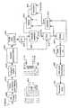
図３は、時間ドメイン補間及び周波数ドメイン補間を含む、本発明の実施形態による補間プロセスの流れ図を示す。チャネル推定器１６０は、ブロック１６１、１６２、１６５を含む。ブロック１６１は、連続パイロット・セルと散乱パイロット・セルを含め、パイロット・セルにおけるチャネル伝達関数を計算する。時間ドメイン補間器１６２は、ブロック１６３と１６４を含む。ブロック１６３は、ＬＭＳアルゴリズムに基づいて時間ドメイン補間器係数更新を計算する。ブロック１６４において、チャネル伝達関数は、すべての散乱パイロット・トーンの非パイロット・セルにおける時間ドメイン補間を使用して計算される。時間ドメイン補間の後、すべての散乱パイロット・トーンにおけるチャネル伝達関数の、時間ドメイン補間を介する推定値又は計算された値が、利用可能である。 FIG. 3 shows a flow diagram of an interpolation process according to an embodiment of the invention, including time domain interpolation and frequency domain interpolation.Channel estimator 160 includesblocks 161, 162, 165.Block 161 calculates the channel transfer function in the pilot cells, including continuous pilot cells and scattered pilot cells.Time domain interpolator 162 includesblocks 163 and 164.Block 163 calculates time domain interpolator coefficient updates based on the LMS algorithm. Atblock 164, the channel transfer function is calculated using time domain interpolation in non-pilot cells of all scattered pilot tones. After time domain interpolation, an estimate or calculated value of the channel transfer function in all scattered pilot tones via time domain interpolation is available.

周波数ドメイン補間器１６５が、すべての非パイロット・トーンにおけるチャネル伝達関数推定値を計算する。ブロック１６５は、ブロック１６６と１６７を含む。ブロック１６６は、ＬＭＳアルゴリズムに基づいて周波数ドメイン補間器係数更新を計算する。ブロック１６７において、チャネル伝達関数が、すべての非パイロット・トーンにおける周波数ドメイン補間を使用して計算される。周波数ドメイン補間の後、すべてのデータ搬送波におけるすべての伝達関数の推定値が、すべての非パイロット・トーンに関する周波数ドメイン補間、又はすべての散乱パイロット・トーンの非パイロット・セルに関する時間ドメイン補間器を介して利用可能である。それらの結果は、ＦＥＱ１７０に送信されて、ＦＥＱ係数がセットアップされる。 Afrequency domain interpolator 165 calculates channel transfer function estimates for all non-pilot tones.Block 165 includesblocks 166 and 167.Block 166 calculates frequency domain interpolator coefficient updates based on the LMS algorithm. Atblock 167, the channel transfer function is calculated using frequency domain interpolation on all non-pilot tones. After frequency domain interpolation, all transfer function estimates on all data carriers are passed through frequency domain interpolation for all non-pilot tones or time domain interpolator for all scattered pilot tones non-pilot cells. Available. Those results are sent to theFEQ 170 to set up the FEQ coefficients.

IV．補間フィルタ構造
通常、補間フィルタは、ローパス・デジタル・フィルタとして設計される。通過帯域の帯域幅は、補間比に依存する。例えば、ＤＶＢ−Ｔ／ＤＶＢ−Ｈシステムにおける時間ドメイン補間の場合、補間比は、４であり、ローパス・フィルタの通過帯域は、ナイキスト周波数の１／４である。ＤＶＢ−Ｔ／ＤＶＢ−Ｈシステムにおける周波数ドメイン補間の場合、補間比は、３であり、ローパス・フィルタの通過帯域は、ナイキスト周波数の１／３である。ローパス・フィルタは、通常、中央タップのまわりに対称的な実係数を使用して実施される。したがって、セクションIIで説明した時間ドメイン補間フィルタの場合、Ｍ１＝Ｍ２であり、セクションIIIにおける周波数ドメイン補間の場合、Ｊ１＝Ｊ２である。IV. Interpolation filter structure The interpolation filter is usually designed as a low-pass digital filter. The bandwidth of the pass band depends on the interpolation ratio. For example, in the case of time domain interpolation in a DVB-T / DVB-H system, the interpolation ratio is 4, and the pass band of the low-pass filter is 1/4 of the Nyquist frequency. For frequency domain interpolation in the DVB-T / DVB-H system, the interpolation ratio is 3, and the passband of the low pass filter is 1/3 of the Nyquist frequency. Low pass filters are typically implemented using real coefficients that are symmetric around the center tap. Thus, for the time domain interpolation filter described in Section II, M1 = M2, and for frequency domain interpolation in Section III, J1 = J2.

しかし、時間ドメイン補間において、以下のとおりのフィルタ・オペレーションを有する（第１のフィルタを例にとる）（セクションII参照）。すなわち、
H(n,ki)＝ΣW1(n,m)H(n-1+4m,ki)(m=-M1+1,-M1+2,...-1,0,1,..M2)
である。However, in time domain interpolation, it has the following filter operations (take the first filter as an example) (see Section II): That is,
H (n, ki) = ΣW1 (n, m) H (n-1 + 4m, ki) (m = -M1 + 1, -M1 + 2, ...- 1,0,1, .. M2)
It is.

０＜ｍ≦Ｍ２に関して、ｎ−１＋４ｍ＞である。したがって、Ｈ（ｎ，ｋｉ）を計算するのに、「将来の」チャネル伝達関数を必要とする。これは、４（Ｍ１＋Ｍ２）個のシンボルに関する連続パイロット・トーン及び散乱パイロット・トーンにおけるすべてのＨ値、及びすべてのデータ搬送波に関する４Ｍ２個のシンボルに関するすべての受信信号Ｙ（ｎ，ｋ）を格納することを要求する。搬送波の数は、極めて大きいので（ＤＶＢ−Ｔにおいて８ｋまで）、これは、相当に大きいメモリ空間を要求する。メモリ要件を小さくするため、Ｍ２を減らすことが望ましい。 For 0 <m ≦ M2, n−1 + 4m>. Therefore, a “future” channel transfer function is required to calculate H (n, ki). This stores all H values in continuous and scattered pilot tones for 4 (M1 + M2) symbols and all received signals Y (n, k) for 4M2 symbols for all data carriers. Request that. Since the number of carriers is very large (up to 8k in DVB-T), this requires a considerable amount of memory space. It is desirable to reduce M2 to reduce memory requirements.

一実施形態では、Ｍ２＜Ｍ１である複素非対称補間フィルタが使用される。複素フィルタは、タイプ当たりの計算を２倍にするものの、パフォーマンスを向上させて、タップの数を減らすのに役立ち、特にＭ２を減らすのに役立つ。さらにメモリ要件を減らすのに、Ｍ２は、フィルタのいくつかに関して０であることさえ可能である。例えば、Ｍ２が、第１のフィルタに関して０であるが、その他の２個のフィルタに関してＭ２＝１である場合、すべてのデータ搬送波に関してわずか３つのシンボルを格納すればよい。 In one embodiment, a complex asymmetric interpolation filter with M2 <M1 is used. Although the complex filter doubles the calculation per type, it improves performance and helps reduce the number of taps, and in particular helps reduce M2. To further reduce memory requirements, M2 can even be zero for some of the filters. For example, if M2 is 0 for the first filter but M2 = 1 for the other two filters, only 3 symbols need be stored for all data carriers.

周波数ドメイン補間において、補間フィルタへのすべての入力は、同一のシンボル内にある。「将来の格納」問題は、まったく存在しない。主な問題は、境界にある。Ｊ１＝Ｊ２である場合、計算される搬送波の各側で３Ｊ１の搬送波と３Ｊ２の搬送波を必要とする。このことは、補間フィルタに利用可能な搬送波が十分に存在しない境界以外は問題ではない。その結果、Ｈの推定が両端で劣化する。この問題を解決するのに、小さいＪ１、又は小さいＪ２（１ほどに小さい）を有する非対称フィルタを使用することが望ましい。これは、複素フィルタを使用することによって可能にされる。 In frequency domain interpolation, all inputs to the interpolation filter are in the same symbol. There is no “future storage” problem. The main problem is at the border. If J1 = J2, then 3J1 and 3J2 carriers are required on each side of the calculated carrier. This is not a problem except for boundaries where there are not enough carriers available for the interpolation filter. As a result, the estimation of H deteriorates at both ends. To solve this problem, it is desirable to use an asymmetric filter with a small J1 or a small J2 (as small as 1). This is made possible by using a complex filter.

補間フィルタは、最悪ケースの条件に基づいて事前設計可能である。例えば、時間ドメイン補間の場合、フィルタは、最高のドップラー周波数を範囲に含まなければならず、周波数ドメイン補間の場合、フィルタは、最長の遅延拡散を範囲に含まなければならない。補間フィルタの阻止帯域は、良好な補間精度と雑音除去を確実にするのに十分なだけの減衰を有さなければならない。雑音は、通常、白色であり、すべての周波数を範囲に含むことに留意されたい。フィルタの通過帯域が、全帯域幅の１／３である場合、雑音の２／３は、阻止帯域内にあり、このため、除去可能である。このため、雑音を除去するのに、補間フィルタ通過帯域は、ドップラー周波数又は遅延拡散が範囲に含まれることが可能である限り、できるだけ狭くなければならない。他方、深い阻止帯域減衰は、補間フィルタ・リソースに重い負担をかける。このため、阻止帯域除去は深すぎてはならないが、パフォーマンス低下が無視できるほどであることを確実にするのに十分なだけちょうどの深さでなければならない。 The interpolation filter can be pre-designed based on worst case conditions. For example, for time domain interpolation, the filter must cover the highest Doppler frequency, and for frequency domain interpolation, the filter must cover the longest delay spread. The stopband of the interpolation filter must have sufficient attenuation to ensure good interpolation accuracy and noise removal. Note that the noise is typically white and covers all frequencies. If the filter passband is 1/3 of the total bandwidth, 2/3 of the noise is in the stopband and can therefore be removed. Thus, to remove noise, the interpolation filter passband must be as narrow as possible as long as the Doppler frequency or delay spread can be included. On the other hand, deep stopband attenuation places a heavy burden on the interpolation filter resources. Thus, stopband rejection should not be too deep, but just deep enough to ensure that performance degradation is negligible.

移動環境の場合、ドップラー周波数、遅延拡散、チャネル雑音条件は、頻繁に変化する。事前設計された補間フィルタは、急速に変化する環境に対して、決して最適化されていない。本発明による適応補間フィルタが、あらゆるチャネル条件の下で、最適なパフォーマンスのための最適なフィルタ設定の理想的な解決を提供する。 In a mobile environment, Doppler frequency, delay spread, and channel noise conditions change frequently. Pre-designed interpolation filters are never optimized for rapidly changing environments. The adaptive interpolation filter according to the present invention provides an ideal solution for optimal filter settings for optimal performance under all channel conditions.

実際の無線通信環境において、ドップラー周波数、遅延拡散、チャネル雑音条件は、必ずしもすべて最悪の条件にあるわけではない。補間フィルタは、主にフィルタ長（複雑度）制約のため、限られたリソースを有する。本発明による適応補間は、補間フィルタが補間フィルタの設定を最適化して、任意の特定の急速に変化するチャネル条件下でシステム・パフォーマンスを最適化することを可能にする。 In an actual wireless communication environment, the Doppler frequency, delay spread, and channel noise conditions are not necessarily all in the worst conditions. Interpolation filters have limited resources mainly due to filter length (complexity) constraints. The adaptive interpolation according to the present invention allows the interpolation filter to optimize the interpolation filter settings to optimize system performance under any particular rapidly changing channel conditions.

複素フィルタ係数の使用により、一部のチャネル条件に関して最適である可能性がある非対称的なフィルタ応答が可能になる。例えば、マルチパス遅延拡散に関して、第１のパスを始まりとして選択して、その他のパスからの信号が、サイクリック・プレフィックスによって扱われることが可能であるようにしなければならない。このことは、他のすべてのパスがより長い遅延を有し、そのため、遅延拡散が片側であることを意味する。その場合、最適な補間フィルタ応答は、片側でなければならない。これは、複素係数を使用し、係数をオンラインで調整することによって可能になる。片側の応答は、雑音の影響を減らして、両側の応答を有する補間フィルタが範囲に含むことができる最大遅延拡散の２倍の大きさの遅延拡散の補正を可能にすることに役立つ（図４及び図５参照）。 The use of complex filter coefficients allows for an asymmetric filter response that may be optimal for some channel conditions. For example, for multipath delay spread, the first path must be selected as the beginning so that signals from other paths can be handled by the cyclic prefix. This means that all other paths have longer delays, so the delay spread is unilateral. In that case, the optimal interpolation filter response must be one-sided. This is made possible by using complex coefficients and adjusting the coefficients online. One-sided response helps to reduce the effects of noise and allow correction of delay spread twice as large as the maximum delay spread that an interpolation filter with two-sided response can cover (FIG. 4). And FIG. 5).

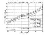
図６、図７は、ＬＭＳ適応アルゴリズムと、最悪ケースのドップラー周波数のために設計された固定の係数とを使用する時間ドメイン補間器のパフォーマンスを比較する。図６では５０Ｈｚという比較的低いドップラー周波数が使用され、図７では１５０Ｈｚという比較的高いドップラー周波数が使用される。補間器の長さは、１７、２５、又は３３である。 FIGS. 6 and 7 compare the performance of time domain interpolators using LMS adaptation algorithms and fixed coefficients designed for the worst case Doppler frequency. In FIG. 6, a relatively low Doppler frequency of 50 Hz is used, and in FIG. 7 a relatively high Doppler frequency of 150 Hz is used. The length of the interpolator is 17, 25 or 33.

図８、図９は、ＬＭＳ適応アルゴリズムと、最悪ケースの遅延拡散のために設計された固定の係数とを使用する周波数ドメイン補間器のパフォーマンスを比較する。図８では、［００．２０．５１．６２．３５．０］μＳという比較的小さい遅延拡散が、使用され、図９では、｛［００．２０．５１．６２．３５．０］μＳ，［００．２０．５１．６２．３５．０］＋５０μＳ，［００．２０．５１．６２．３５．０］＋１００μＳ｝という大きい遅延拡散が、使用される。補間器の長さは、２１、２７、又は３３である。 FIGS. 8 and 9 compare the performance of frequency domain interpolators using LMS adaptation algorithms and fixed coefficients designed for worst-case delay spread. In FIG. 8, a relatively small delay spread of [0 0.2 0.5 1.6 1.6 5.0] μS is used, and in FIG. 9, {[0 0.2 0.5 0.5 1.6 2.3 5.0] μS, [0 0.2 0.5 1.6 2.3 5.0] +50 μS, [0 0.2 0.5 1.6 2.3 5.0] +100 μS} A large delay spread is used. The length of the interpolator is 21, 27, or 33.

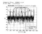
図１０は、１２ｄＢ入力ＳＮＲと２１のタップにおける片側の遅延拡散｛［００．２０．５１．６２．３５．０］μＳ，［００．２０．５１．６２．３５．０］＋５０μＳ，［００．２０．５１．６２．３５．０］＋１００μＳ｝を有する周波数ドメインＬＭＳ適応補間器の応答を示す。また、補間器への入力のＦＦＴも、青で示されている。右から最初の３つのピークが、３つの遅延グループを表す。ＬＭＳ補間器は、それら２つのピークが通過することを許す。その他すべてのピークは、ＬＭＳ適応補間器の無効に入っており、そのため、除去される。 FIG. 10 shows 12 dB input SNR and one side delay spread at 21 taps {[0 0.2 0.5 1.6 2.3 5.0] μS, [0 0.2 0.5 1.6 2. 2 shows the response of a frequency domain LMS adaptive interpolator with 3 5.0] +50 μS, [0 0.2 0.5 1.6 2.3 5.0] +100 μS}. The FFT of the input to the interpolator is also shown in blue. The first three peaks from the right represent three delay groups. The LMS interpolator allows these two peaks to pass. All other peaks have entered the LMS adaptive interpolator disabled and are therefore removed.

図１１は、時間ドメインＬＭＳ適応補間器、固定補間器、フィルタ入力のＦＦＴを示す。５０Ｈｚという適度のドップラー周波数が、１２ｄＢの入力信号ＳＮＲで使用される。２５のフィルタ・タップが使用される。通過帯域は、適応補間器において、ドップラーがより低いので、固定の元のフィルタよりも狭いことに留意されたい。このより狭い通過帯域は、より少ない雑音が通過することを許し、そのため、パフォーマンスを向上させる。適応補間器における阻止帯域減衰は、このケースに関して、ちょうど十分な減衰を得るように緩和される。元の補間器におけるより深い減衰は必要ではなく、鋭いフィルタは、しばしば、他の問題を生じさせ、パフォーマンスを低下させる。明らかに、適応フィルタは、利用可能なフィルタ・リソースを最適に使用して、出力平均２乗誤差を最小限に抑えることができる。 FIG. 11 shows the time domain LMS adaptive interpolator, fixed interpolator, and filter input FFT. A moderate Doppler frequency of 50 Hz is used with an input signal SNR of 12 dB. 25 filter taps are used. Note that the passband is narrower than the fixed original filter in the adaptive interpolator due to the lower Doppler. This narrower passband allows less noise to pass, thus improving performance. The stopband attenuation in the adaptive interpolator is relaxed to obtain just enough attenuation for this case. Deeper attenuation in the original interpolator is not necessary, and a sharp filter often creates other problems and degrades performance. Clearly, the adaptive filter can optimally use available filter resources to minimize the output mean square error.

図１２は、５０Ｈｚのドップラー周波数の下で非対称時間ドメイン複素フィルタを示す。この非対称フィルタでは、わずか１つの「将来の」Ｈ値しか必要とされず、そのため、「将来の」シンボルのためのストレージがはるかに縮小される。図１１は、そのようなフィルタ、及びそのようなフィルタの入力のＦＦＴを示す。 FIG. 12 shows an asymmetric time domain complex filter under a 50 Hz Doppler frequency. With this asymmetric filter, only one “future” H value is required, so the storage for “future” symbols is much reduced. FIG. 11 shows an FFT of such a filter and the input of such a filter.

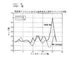
図１４、図１５は、非対称周波数ドメイン補間器を示す。遅延拡散｛［００．２０．５１．６２．３５．０］μＳ，［００．２０．５１．６２．３５．０］＋５０μＳ，［００．２０．５１．６２．３５．０］＋１００μＳ｝が、１２ｄＢの入力ＳＮＲ、及び２１のタップにおいて使用される。非対称周波数ドメイン補間器は、図１６に示される境界効果を減らすことに役立つ。この適応補間の収束が、図１７に示される。 14 and 15 show an asymmetric frequency domain interpolator. Delay spread {[0 0.2 0.5 1.6 2.3 5.0] μS, [0 0.2 0.5 1.6 2.3 5.0] +50 μS, [0 0.2 0. 5 1.6 2.3 5.0] +100 μS} is used at an input SNR of 12 dB and 21 taps. The asymmetric frequency domain interpolator helps reduce the boundary effects shown in FIG. The convergence of this adaptive interpolation is shown in FIG.

以上は、本発明の様々な実施形態の詳細な説明を提供したが、多くの代替形態、変形形態、及び等価形態が可能である。例えば、適応チャネル推定のいくつかの実施形態を、ＤＶＢ−Ｔ及びＤＶＢ−Ｈの文脈で説明したが、本発明による適応チャネル推定は、他の無線標準の実施形態において使用されることも可能である。したがって、本発明の範囲は、説明した実施形態に限定されるべきではなく、代わりに、添付の特許請求の範囲によって定義される。 Although the foregoing has provided a detailed description of various embodiments of the invention, many alternatives, modifications, and equivalents are possible. For example, although some embodiments of adaptive channel estimation have been described in the context of DVB-T and DVB-H, adaptive channel estimation according to the present invention can also be used in other wireless standard embodiments. is there. Accordingly, the scope of the invention should not be limited to the described embodiments, but instead is defined by the appended claims.

ＯＦＤＭベースの無線受信機のブロック図である。1 is a block diagram of an OFDM-based wireless receiver.ＤＶＢ−Ｔ及びＤＶＢ−Ｈにおけるパイロット挿入パターンを示す図である。It is a figure which shows the pilot insertion pattern in DVB-T and DVB-H.補間器ベースのチャネル推定器を示すブロック図である。FIG. 6 is a block diagram illustrating an interpolator-based channel estimator.両側信号の３による補間を示す図である。It is a figure which shows the interpolation by 3 of a both-sides signal.片側信号の３による補間を示す図である。It is a figure which shows the interpolation by 3 of the one-side signal.時間ドメイン補間器パフォーマンス（５０Ｈｚドップラー）を示すプロットである。FIG. 6 is a plot showing time domain interpolator performance (50 Hz Doppler). FIG.時間ドメイン補間器パフォーマンス（１５０Ｈｚドップラー）を示すプロットである。FIG. 6 is a plot showing time domain interpolator performance (150 Hz Doppler). FIG.周波数ドメイン補間器パフォーマンス（小さい拡散）を示すプロットである。Fig. 6 is a plot showing frequency domain interpolator performance (small diffusion).周波数ドメイン補間器パフォーマンス（大きい拡散）を示すプロットである。Figure 5 is a plot showing frequency domain interpolator performance (large spread).周波数ドメインＬＭＳ適応補間器係数のＦＦＴ、及び入力を示すプロットである。FIG. 5 is a plot showing FFT and input of frequency domain LMS adaptive interpolator coefficients. FIG.時間ドメインＬＭＳ適応補間器係数のＦＦＴ、固定補間器係数、及びフィルタ入力を示すプロットである。FIG. 6 is a plot showing FFT of time domain LMS adaptive interpolator coefficients, fixed interpolator coefficients, and filter input. FIG.非対称時間ドメイン適応補間器係数を示すプロットである。Figure 5 is a plot showing asymmetric time domain adaptive interpolator coefficients.非対称時間ドメイン適応補間器係数のＦＦＴ、及び入力を示すプロットである。FIG. 6 is a plot showing FFT and input of asymmetric time domain adaptive interpolator coefficients. FIG.非対称周波数ドメイン適応補間器係数を示すプロットである。Figure 5 is a plot showing asymmetric frequency domain adaptive interpolator coefficients.非対称周波数ドメイン適応補間器係数のＦＦＴ、及び入力を示すプロットである。FIG. 6 is a plot showing FFT and input of asymmetric frequency domain adaptive interpolator coefficients. FIG.境界効果を減らすのに役立つ非対称周波数ドメイン適応補間器を示すプロットである。Figure 5 is a plot illustrating an asymmetric frequency domain adaptive interpolator that helps reduce boundary effects.非対称周波数ドメイン補間の収束を示すプロットである。Fig. 6 is a plot showing the convergence of asymmetric frequency domain interpolation.本発明の実施形態によるＯＦＤＭベースの無線受信機を示すブロック図である。FIG. 2 is a block diagram illustrating an OFDM-based wireless receiver according to an embodiment of the present invention.