EP0379399A1 - Process for calculating and evaluating a conically projected image, for example an X-ray image, of a three-dimensional sampled object, and process for the three-dimensional reconstruction of an object subject to above calculating process - Google Patents
Process for calculating and evaluating a conically projected image, for example an X-ray image, of a three-dimensional sampled object, and process for the three-dimensional reconstruction of an object subject to above calculating processDownload PDFInfo
- Publication number
- EP0379399A1 EP0379399A1EP90400083AEP90400083AEP0379399A1EP 0379399 A1EP0379399 A1EP 0379399A1EP 90400083 AEP90400083 AEP 90400083AEP 90400083 AEP90400083 AEP 90400083AEP 0379399 A1EP0379399 A1EP 0379399A1
- Authority
- EP
- European Patent Office
- Prior art keywords
- function
- functions
- sampled
- basic
- projection
- Prior art date
- Legal status (The legal status is an assumption and is not a legal conclusion. Google has not performed a legal analysis and makes no representation as to the accuracy of the status listed.)
- Granted
Links
Images

Classifications
- G—PHYSICS
- G06—COMPUTING OR CALCULATING; COUNTING
- G06T—IMAGE DATA PROCESSING OR GENERATION, IN GENERAL
- G06T11/00—2D [Two Dimensional] image generation
- G06T11/003—Reconstruction from projections, e.g. tomography
- G06T11/006—Inverse problem, transformation from projection-space into object-space, e.g. transform methods, back-projection, algebraic methods
- G—PHYSICS
- G06—COMPUTING OR CALCULATING; COUNTING
- G06T—IMAGE DATA PROCESSING OR GENERATION, IN GENERAL
- G06T2211/00—Image generation
- G06T2211/40—Computed tomography
- G06T2211/424—Iterative
Definitions
- the subject of the present inventionis a method for calculating and exploiting the image in conical projection, for example in the X-ray sense, of a three-dimensional (3D) object sampled in volume elements, as well as a method of three-dimensional reconstruction of a studied object using this calculation process.
- the inventionfinds its use more particularly in the medical field where the objects studied are the bodies of patients subjected to a radiological examination. To this end, it essentially concerns three-dimensional reconstruction. However, it would also be applicable to two-dimensional reconstruction methods. Likewise, it can be used for viewing a sampled volume.
- the object of the inventionis to contribute to the production of representative images of 3D objects studied which are both sharper and obtained more quickly.
- Two-dimensional (2D) reconstructions of images of sections of objectsare known after acquisitions (1D) in radiological computed tomography performed in the section to be imaged.
- the different generations of CT scannershave led to the use, in a third generation, of fan beam X-ray CT scanners, in which a point X-ray source illuminates a so-called multidetector detector in X-ray, comprising a plurality of cells aligned in the plane of the fan beam.
- the object to be studiedis interposed between the X-ray source and the multidetector.
- the acquisitionincludes a series of illuminations. From one illumination to another, the X-multidetector source assembly is turned around the body to be studied.
- the acquisition timeis of the order of four seconds.
- the acquisitions necessary for 256 cutswould then lead to an examination time close to half an hour. This period is far too long to bear for patients and for the health system in general (cost).
- RADON theoryleads to the acquisition of measures corresponding to the integration of the physical characteristics to be imaged in a set of subspace, called hyperplanes, whose dimension is one unit smaller than the dimension of the space studied and to rebuild. In other words, for a 3D studied space it is necessary to have measurement results integrated on 2D hyperplanes.
- the radiological acquisition with point detectorcan only be an integration of the characteristics on a straight line (1 D): the X-ray.
- the trajectory of the sourcedoes not respect the conditions fixed by theory, it will not be possible, on the sole knowledge of the projections along the set of straight lines (X-rays) used for the acquisition, to calculate the projections according to all the hyperplanes necessary for the reconstruction.
- pointswill be missing in the Radon space of the measurements. This will not be filled on a regular basis. The consequence is the appearance of artifacts in the resulting 3D reconstructions.
- f jrepresents the absorption function in each of the voxels (the volume elements sampled) crossed
- This weightingmay be approximated by the length of the intersection between the crossed voxel and the X-ray.
- the results providedare unfortunately of insufficient quality for the applications envisaged.
- a jultimately represents the description of the function f sought, the b j (x, y, z) being known.
- the operation of projecting the estimate 7 of famounts to calculating In this expression g ; denotes a weighting function with zero (or very low) value outside the angular sector formed by the source s and the cell i.
- the g functionsare representative of the conical illumination support of cell i.
- Each weight h ijtranslates the contribution of the basic function b j to the projection of the object on cell i.
- the object of the inventionis therefore to allow, from the knowledge of samples f i of a function f of three variables, the numerical calculation of the projection of f on a detector cell i, by ensuring both a good quality of the result obtained, and very short calculation times.
- quality and speedare essential in the reconstruction of a function f (x, y, z) from a set of 2D conic projections using algebraic reconstruction techniques. While the projection methods of the state of the art do not make it possible to ensure both the quality and the speed desired, the invention will allow it.
- FIG. 1represents a source S of X-rays which illuminates a body C so that detector cells i of a multidetector D measure the attenuation of this illumination after passing through the body C.
- the multidetector usedis a plane (as the exterior surface of a radiological luminance intensifying screen is comparable to a plane).
- a concave multidetectoras would be a silicon multidetector provided with photodetector cells.
- Such a concave multidetectoris at all points on its surface perpendicular to the conical X-ray which illuminates it.
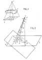
- Figure 2shows three direct orthonormal landmarks.
- a first orthonormal reference frame x, y, zis integral with the body C.
- the detector Dassumed to be plane is characterized by a central point noted P which is the orthogonal projection of the source S on the plane of this multidetector.
- a reference x, y, z attached to the detector Dis then characterized by the fact that z 'is co-linear, and in the same direction, as SP while x and y', to simplify oriented along the orthogonal edges of the detector D, form with z 'a direct orthonormal reference.
- Cell iis assumed to be a square on the plane of detector D.
- the orthonormal vectors x; and y;are orthogonal to z i , the vector x i being contained in the plane of the detector D.
- the radius SP iis perpendicular to a plane ⁇ i containing the vector x i .
- G ⁇ ab (u)denotes a truncated Gaussian standard deviation ⁇ b such that:
- R b3 ⁇ x / 2.
- the weighting function gmust be non-negative inside the polyhedron with vertex S and base cell i, and almost zero outside this polyhedron.
- the weight assigned to each of the planes z i(plane orthogonal to the axis FP i ) must be the same since each of these planes is cut by the same number of rays coming from the source. This constraint results in the fact that the integral evaluated in the coordinate system xi, yi, zi attached to cell i must be independent of z k .
- g-weighting functionsare Gaussian.
- theyare even truncated Gaussian.
- these functionsare 2D Gaussians. But in 3D space these are not Gaussian functions.
- FIG. 3shows a schematic representation of the restriction, in the plane of the detector D of one of these weighting functions.
- This restrictionis, to a very slight approximation, a truncated 2D Gaussian.
- the center of this Gaussianis P i
- its standard deviationis ⁇ g
- its truncation radiusis Rg.
- the standard deviation ⁇ g and the radius Rgcan be chosen by the user.
- it may be more convenient, to give the mathematical expression of g ito be placed in the reference frame of the cell (x i , y i , z i ).
- G ⁇ (u)is a truncated 1 D Gaussian such that if
- ⁇ R gx (zk) and such that G ⁇ gx (zk ) (xk)0 if
- G ⁇ gy (zk)in the same way.
- Rg xis the truncation radius on the axis x i
- Rgyis similarly the truncation radius on the axis y i ).
- the Gaussiansare in fact parameterized by z k since the standard deviations depend of course on the altitude of the basic function thus weighted with respect to the source S, due to the conical nature of the projection. For this reason the standard deviations ag x (Z k ) and ⁇ gy (Z k ) are defined by
- the support of g iis a cone with vertex S, axis SP i , and elliptical base (in the plane ⁇ i ).
- the restriction of g ion the detector plane, is no different from a truncated 2D Gaussian, of standard deviation ag (along x 'or y').
- the support of this restrictionis little different from the circle of center P; and of radius Rg.
- Support for this restriction of gis not a perfect circle because in fact the source S is not at infinity. Indeed if the source S was at infinity, and if its projection in the plane ⁇ i was effectively elliptical, its projection in the plane of the detector would be strictly a circle.
- the projectionis conical, the projected circle is a little distorted: the resulting error is of the second order. It can be overlooked.
- the function gthus chosen satisfies the constraint that is independent of z i . Indeed this double sum can be written: which is a constant. The equality is not exact because instead of being pure Gaussians the Gaussian functions used are truncated.
- a standard deviation of the weighting functionsuch that the width at mid-height of the Gaussians is equal to the width of a voxel (in the attached frame and at l location of the detector cell).
- FIG. 4shows the local domain of definition of the function b j limited around the point V j . This domain is a circle limited by the radius R b (R b being the truncation radius of the Gaussian defining b j ).
- Figure 4illustrates the integration proposed by the formula 11.
- This part of the supportis normally a truncated cone, elliptical, the largest base of which is fixed by the altitude z j - R b and the smallest base of which is fixed by the altitude z j + R b .
- R bis also small (by assumption of the "local" bases)
- each of the two integrals of this last expressioncan be interpreted as a convolution product of two centered Gaussians.
- the convolution product of two centered Gaussiansis known to be an equally centered Gaussian, the variance of which is equal to the sum of the two variances of the starting Gaussians. This then leads to the particularly simple expression, after calculation, and either for P; (f):
- the values x i and y j appearing in equation 30are, for each cell 1, coordinates of the voxels relative to the frame of reference cell i.
- the values x j and y j appearing in equation 30are, in the reference frame cell i, the abscissa and the ordinate of the center V j of the function of the base b j .
- the coordinates of P i V jare noted (x ' j , y' j ).
- the vector P i V j 'is equal to the projection, on the plane of the detector and in the direction SP i , of the vector of coordinates (x j , y j ).
- the invented algorithmcan allow, knowing a correctly sampled function f to propose images in conical projection according to a main direction SP to be defined .
- the advantage of the inventionis then to provide an image without artifact obtained more quickly than in the state of the art. Choosing a Gaussian weighting function, whose standard deviation is (and this with all the simplifications presented) still a function of the altitude of the basic function normally leads to a weighting naturally adapted to the conical nature of the illumination . In this way we decrease the artifacts and speed up the reconstruction.
- the inventionnaturally relates to all the operations made of the images or calculated reconstructions. These operations notably include the visualization of reconstructed structures or calculated images.
Landscapes
- Physics & Mathematics (AREA)
- Engineering & Computer Science (AREA)
- Theoretical Computer Science (AREA)
- General Physics & Mathematics (AREA)
- Mathematical Physics (AREA)
- Mathematical Optimization (AREA)
- Mathematical Analysis (AREA)
- Pure & Applied Mathematics (AREA)
- Algebra (AREA)
- Image Analysis (AREA)
- Apparatus For Radiation Diagnosis (AREA)
- Image Processing (AREA)
- Image Generation (AREA)
- Analysing Materials By The Use Of Radiation (AREA)
Abstract
Translated fromFrenchDescription
Translated fromFrenchLa présente invention a pour objet un procédé de calcul et d'exploitation de l'image en projection conique, par exemple au sens des rayons X, d'un objet tridimensionnel (3D) échantillonné en éléments de volume, ainsi qu'un procédé de reconstruction tridimensionnelle d'un objet étudié utilisant ce procédé de calcul. L'invention trouve son utilisation plus particulièrement dans le domaine médical où les objets étudiés sont des corps de patients soumis à un examen radiologique. Dans ce but, elle concerne essentiellement la reconstruction tridimensionnelle. Cependant, elle serait également applicable à des procédés de reconstruction bidimensionnelle. De même elle est utilisable en visualisation d'un volume échantillonné. Le but de l'invention est de concourir à la production d'images représentatives d'objet 3D étudiés qui soient à la fois plus nettes et obtenues plus rapidement.The subject of the present invention is a method for calculating and exploiting the image in conical projection, for example in the X-ray sense, of a three-dimensional (3D) object sampled in volume elements, as well as a method of three-dimensional reconstruction of a studied object using this calculation process. The invention finds its use more particularly in the medical field where the objects studied are the bodies of patients subjected to a radiological examination. To this end, it essentially concerns three-dimensional reconstruction. However, it would also be applicable to two-dimensional reconstruction methods. Likewise, it can be used for viewing a sampled volume. The object of the invention is to contribute to the production of representative images of 3D objects studied which are both sharper and obtained more quickly.
On connaît les reconstructions à deux dimensions (2D) d'images de coupes d'objets après des acquisitions (1D) en tomodensitométrie radiologique effectuées dans la coupe à imager. Les différentes générations de tomodensitomètres ont conduit à l'utilisation, en une troisième génération, des tomodensitomètres à faisceau de rayons X en éventail (fan beam), dans lesquels une source de rayons X ponctuelle illumine en rayonnement X un détecteur dit multidétecteur, comportant une pluralité de cellules alignées dans le plan du faisceau en éventail. L'objet à étudier est interposé entre la source à rayons X et le multidétecteur. L'acquisition comporte une série d'illuminations. D'une illumination à une autre l'ensemble source à rayons X-multidétecteur est tourné autour du corps à étudier. Si on appelle s la coordonnée longitudinale d'une cellule du multidétecteur sur ce multidétecteur, et si on appelle e l'angle de repérage de l'ensemble source à rayons X -multidétecteur au moment de l'illumination, on obtient de cette manière une série de mesures d'absorption radiologique notée P(e,s). Si on appelle x et y les coordonnées d'un élément de volume de l'objet à étudier, dans la coupe concernée, et si on note f(x, y,) la fonction d'atténuation linéaire du rayonnement X qui passe à travers l'objet, on peut écrire :
L'application des théories de RADON avait conduit à rechercher la transformée de FOURIER monodi- mensionnelle de P(8,s) notée P e(u). En recherchant ensuite la transformée de FOURIER bidimensionnelle de f(x, y) notée F(v,w), on pouvait être conduit à identifier P θ (u) et F (v, w) évaluées sur la droite d'angle 8. On en a déduit que par une transformée de FOURIER bidimensionnelle inverse de f (v,w) obtenue à partir de l'ensemble des P θ (u) (après changement de variables et interpolation), on pouvait calculer la distribution de f(x,y) dans la coupe étudiée à partir des mesures P(8,s).The application of RADON theories had led to the search for the monodimensional FOURIER transform of P (8, s) denoted P e (u). By then looking for the two-dimensional FOURIER transform of f (x, y) denoted F (v, w), we could be led to identify P θ (u) and F (v, w) evaluated on the line of angle 8. We deduced that by an inverse two-dimensional FOURIER transform of f (v, w) obtained from the set of P θ (u) (after change of variables and interpolation), we could calculate the distribution of f (x , y) in the section studied from the measurements P (8, s).
En pratique, on évite les transformées de FOURIER qui conduisent à des calculs trop longs et utilise une technique dite de filtrage suivie de rétroprojection. Le filtrage consiste à calculer le produit de convolution de la fonction P(8,s), représentative des mesures, par une fonction de filtre q(s). Ce produit est le suivant :
Jusqu'à présent l'acquisition d'informations et la reconstruction 3D des structures examinées est effectuée en déplaçant en translation l'ensemble source à rayons X - multidétecteur le long du corps à étudier et en acquérant ainsi une pluralité d'images de coupe 2D adjacentes dans ce corps. Cependant cette technique est complètement déconseillée en angiographie où, pour obtenir du contraste sur les vaisseaux sanguins, on injecte un produit de constraste. L'injection de ce produit de contraste est traumatisante pour le patient surtout dans la mesure où elle est répétée trop souvent. Il est par exemple prohibé d'effectuer 256 injections de produit de contraste si on veut acquérir des images de 256 coupes adjacentes dans le corps. Outre cette prohibition dans les images d'angiographie, il faut reconnaître que la technique d'acquisition 2D et de reconstruction 2D correspondante est trop longue à mettre en oeuvre pour reconstruire les objets 3D. En effet, avec une résolution moyenne de 256 points par 256 points dans une image de coupe, la durée d'acquisition, avec un tomodensitomètre actuel, est de l'ordre de quatre secondes. Les acquisitions nécessaires à 256 coupes conduiraient alors à une durée d'examen proche de la demie heure. Cette durée est bien trop longue à supporter pour les patients et pour le système de santé en général (coût).Up to now, the acquisition of information and the 3D reconstruction of the structures examined has been carried out by moving the X-ray source - multidetector assembly in translation along the body to be studied and thereby acquiring a plurality of 2D section images. adjacent in this body. However, this technique is completely discouraged in angiography where, to obtain contrast on the blood vessels, a contrast product is injected. The injection of this contrast product is traumatic for the patient, especially since it is repeated too often. It is, for example, prohibited to perform 256 injections of contrast product if one wishes to acquire images of 256 adjacent sections in the body. In addition to this prohibition in angiography images, it must be recognized that the 2D acquisition and corresponding 2D reconstruction technique is too long to implement to reconstruct 3D objects. Indeed, with an average resolution of 256 points by 256 points in a cut image, the acquisition time, with a current CT scanner, is of the order of four seconds. The acquisitions necessary for 256 cuts would then lead to an examination time close to half an hour. This period is far too long to bear for patients and for the health system in general (cost).
En théorie il est possible de généraliser la méthode de RADON en procédant à des acquisitions 3D et en effectuant directement la reconstruction 3D des objets à étudier. Par reconstruction 3D on entend le calcul d'un volume numérique dans lequel des cellules mémoires, placées à des adresses représentatives des voxels du volume étudié, contiennent une information correspondant à la distribution du phénomène (radiologique) étudié dans l'objet. Cependant, la théorie de RADON conduit à acquérir des mesures correspondant à l'intégration des caractéristiques physiques à imager dans un ensemble de sous-espace, dits hyperplans, dont la dimension est d'une unité inférieure à la dimension de l'espace étudié et à reconstruire. Autrement dit, pour un espace étudié 3D il faut disposer de résultats de mesure intégrés sur des hyperplans 2D. Or l'acquisition radiologique avec détecteur ponctuel ne peut être qu'une intégration des caractéristiques sur une droite (1 D) : le rayon X. Dans la mesure où en pratique la trajectoire de la source ne respecte pas les conditions fixées par la théorie, il ne sera pas possible, à partir de la seule connaissance des projections suivant l'ensemble des droites (rayons X) ayant servi à l'acquisition, de calculer les projections selon tous les hyperplans nécessaires à la reconstruction. Autrement dit il manquera des points dans l'espace de Radon des mesures. Celui-ci ne sera pas remplit d'une manière régulière. La conséquence en est l'apparition d'artefacts dans les reconstructions 3D résultantes. Aussi, si des multidé- tecteurs à deux dimensions sont actuellement envisageables (arrangement de photo-détecteurs au silicium, utilisation d'écran intensificateur d'images radiologiques) les reconstructions 3D par cette méthode sont encore à ranger au rang des souhaits devant l'imperfection des résultats auxquels elle conduit quand on ne peut pas lui fournir beaucoup de données, comme c'est le cas dans les applications vasculaires.In theory it is possible to generalize the RADON method by making 3D acquisitions and by directly carrying out the 3D reconstruction of the objects to be studied. By 3D reconstruction is meant the calculation of a digital volume in which memory cells, placed at addresses representative of the voxels of the volume studied, contain information corresponding to the distribution of the (radiological) phenomenon studied in the object. However, RADON theory leads to the acquisition of measures corresponding to the integration of the physical characteristics to be imaged in a set of subspace, called hyperplanes, whose dimension is one unit smaller than the dimension of the space studied and to rebuild. In other words, for a 3D studied space it is necessary to have measurement results integrated on 2D hyperplanes. Now the radiological acquisition with point detector can only be an integration of the characteristics on a straight line (1 D): the X-ray. Insofar as in practice the trajectory of the source does not respect the conditions fixed by theory, it will not be possible, on the sole knowledge of the projections along the set of straight lines (X-rays) used for the acquisition, to calculate the projections according to all the hyperplanes necessary for the reconstruction. In other words, points will be missing in the Radon space of the measurements. This will not be filled on a regular basis. The consequence is the appearance of artifacts in the resulting 3D reconstructions. Also, if two-dimensional multi-detectors are currently possible (arrangement of silicon photo-detectors, use of intensifying screen of radiological images) 3D reconstructions by this method are still to be ranked as desired in the face of imperfection results to which it leads when it cannot be given much data, as is the case in vascular applications.
Il a été envisagé une technique algébrique de reconstruction radicalement différente et basée sur les principes suivants. On connaît l'ensemble des mesures P(θ,τ,s) acquis avec un multidétecteur à deux dimensions, plan ou concave. On sait par ailleurs qu'il existe une fonction continue f(x,y,z) représentative du phénomène d'absorption radiologique qu'on cherche à représenter. On cherche par la reconstruction à connaître f. Dans la pratique compte tenu de ce que tous les calculs sont effectués par des traitements de type informatique, la connaissance de f à l'issue est une connaissance échantillonnée. La nouvelle approche a consisté à estimer f par une fonction discrète notée f fixée à priori. Par exemple f peut au départ consister en un volume numérique où tous les voxels sont fixés à un (ou à zéro). On projette ensuite cette fonction discrète sur le multidétecteur comme si le volume étudié correspondait exactement à cette fonction discrète. On obtient une estimation notéei(f). Ceci peut encore s'écrire

On réitère cet ensemble de projections jusqu'à ce que l'identité de Pi(f) et de Pi(f) soit suffisante. Cette technique a été décrite dans "IMAGES RECONSTRUCTION FROM PROJECTION" G. T. HERMAN ACADEMIC PRESS 1980.We repeat this set of projections until the identity of Pi (f) and Pi (f) is sufficient. This technique has been described in "IMAGES RECONSTRUCTION FROM PROJECTION" G. T. HERMAN ACADEMIC PRESS 1980.
Par ailleurs, si la matrice H de projection est une matrice binaire, avec des 1 et des 0, les résultats sont mauvais. Ainsi une première solution a consisté à approcher P par l'intégrale curviligne de f, prise le long d'une droite D reliant la source S et le centre de chaque cellule sur le multidétecteur. Ceci revient cependant à considérer que chaque cellule est de taille infiniment petite puisque de cette façon on ne prend pas en compte la surface réelle de la cellule, ni le caractère conique de la projection sur cette cellule. Le calcul de cette intégrale curviligne peut se mener de plusieurs manières. La plus simple consiste à approcher l'intégrale curviligne par une somme pondérée des valeurs des voxels traversés par le rayon le rayon X. Ainsi, on pourra écrire
Un autre calcul de pondération a été imaginé : il est décrit dans "AN IMPROVED ALGORITHM FOR REPROJECTING RAYS THROUGH PIXEL IMAGES", par P. M. JOSEPH, IEEE - MI, VOLUME 1, N° 3 PAGES 192-196. L'idée de base de cet autre calcul est d'approcher l'intégrale curviligne de f par une somme portant sur les valeurs interpolées de f prises aux intersections de la droite suivie par le rayon X et de droites horizontales (ou verticales) passant par les centres des voxels visités ou frôlés par le rayon X, ce rayon aboutissant au centre de la cellule du multidétecteur. Les valeurs de f en ces points d'intersection sont estimées au moyen d'une interpolation linéaire entre deux échantillons les plus proches, dans la direction horizontale (ou dans la direction verticale), suivant la pente de la droite du rayon X.Another weighting calculation has been devised: it is described in "AN IMPROVED ALGORITHM FOR REPROJECTING RAYS THROUGH PIXEL IMAGES", by P. M. JOSEPH, IEEE - MI, VOLUME 1, N ° 3 PAGES 192-196. The basic idea of this other calculation is to approach the curvilinear integral of f by a sum relating to the interpolated values of f taken at the intersections of the line followed by the X-ray and of horizontal (or vertical) lines passing through the centers of the voxels visited or grazed by the X-ray, this ray ending at the center of the multidetector cell. The values of f at these intersection points are estimated by means of a linear interpolation between two closest samples, in the horizontal direction (or in the vertical direction), along the slope of the line of the X-ray.
Une généralisation de la méthode des pieds carrés a été proposée par K. M. HANSON and G. W. WECKSUNG, "LOCAL BASIS - FUNCTIONS APPROACH TO COMPUTED TOMOGRAPHY" , APPLIED OPTICS, VOL 24 N° 23, DECEMBRE 1985, PAGES 4028-4039. Dans cette généralisation on construit à partir des échantillons f(xj,yj,zj) une fonction continue f(x,y,z) et on calcule la projection de cette fonction continue sur la cellule i du multidétecteur. Dans cette généralisation la fonction f est définie comme une combinaison linéaire d'un ensemble de fonctions de base b;(x,v,z), et on peut écrire :A generalization of the square feet method was proposed by KM HANSON and GW WECKSUNG, "LOCAL BASIS - FUNCTIONS APPROACH TO COMPUTED TOMOGRAPHY", APPLIED OPTICS, VOL 24 N ° 23, DECEMBER 1985, PAGES 4028-4039. In this generalization, we construct from the samples f (xj , yj , zj ) a continuous function f (x, y, z) and we calculate the projection of this continuous function on cell i of the multidetector. In this generalization the function f is defined as a linear combination of a set of basic functions b; (x, v, z), and we can write:

Dans cette formule aj représente en définitive la description de la fonction f recherchée, les bj(x,y,z) étant connus. On utilise généralement des fonctions de base qui sont locales, répétitives, et séparables. Elles sont locales signifie que le support de chaque fonction bj est petit comparé à celui de f. Elles sont répétitives signifie que chaque fonction bj se déduit par translation d'une unique fonction b(x,y,z). Cette déduction est de la forme

L'opération de projection de l'estimation 7 de f revient à calculer

Le but de l'invention est donc de permettre, à partir de la connaissance d'échantillons fi d'une fonction f de trois variables, le calcul numérique de la projection de f sur une cellule détectrice i, en assurant à la fois une bonne qualité du résultat obtenu, et des temps de calcul très réduits. Ces deux critères (qualité et rapidité) sont essentiels dans la reconstruction d'une fonction f(x,y,z) à partir d'un ensemble de projections coniques 2D au moyen de techniques algébriques de reconstruction. Alors que les méthodes de projection de l'état de la technique ne permettent pas d'assurer à la fois la qualité et la rapidité désirées, l'invention va le permettre.The object of the invention is therefore to allow, from the knowledge of samples fi of a function f of three variables, the numerical calculation of the projection of f on a detector cell i, by ensuring both a good quality of the result obtained, and very short calculation times. These two criteria (quality and speed) are essential in the reconstruction of a function f (x, y, z) from a set of 2D conic projections using algebraic reconstruction techniques. While the projection methods of the state of the art do not make it possible to ensure both the quality and the speed desired, the invention will allow it.
Dans ce but, l'invention a pour objet un procédé de calcul de l'image illuminée en projection conique, par exemple au sens des rayons X, d'un objet tridimensionnel échantillonné en éléments de volume, dans lequel
- - on décompose l'objet tridimensionnel échantillonné sur un espace de fonctions de base gaussiennes,
- - on calcule, pour chaque élément d'image de l'image projetée, des contributions des fonctions de base correspondant aux éléments de volume se projetant sur l'élément d'image considéré, chaque contribution étant égale à l'intégrale du produit de la fonction de base relative à un élément de volume par une fonction représentative d'un support d'illumination de l'élément d'image considéré,
caractérisé en ce que
- - on remplace les fonctions représentatives du support par des fonctions de pondération gaussiennes. L'invention a également pour objet un procédé de reconstruction tridimensionnelle d'un objet étudié, utilisant ce procédé de calcul de manière itérative pour, à partir d'une fonction discrète échantillonnée et à priori représentative de l'objet à reconstruire, retrouver itérativement la fonction f à reconstruire. Dans ce cas l'élément d'image s'identifie avec une cellule d'un multidétecteur 2D.
- - we decompose the three-dimensional object sampled on a space of basic Gaussian functions,
- - For each image element of the projected image, contributions of the basic functions corresponding to the volume elements projecting onto the image element under consideration are calculated, each contribution being equal to the integral of the product of the basic function relating to a volume element by a function representative of an illumination medium for the image element under consideration,
characterized in that
- - the representative functions of the support are replaced by Gaussian weighting functions. The subject of the invention is also a method of three-dimensional reconstruction of a studied object, using this method of calculation in an iterative manner for, from a discrete sampled function and a priori representative of the object to be reconstructed, iteratively find the function f to be reconstructed. In this case the image element is identified with a cell of a 2D multidetector.
L'invention sera mieux comprise à la lecture de la description qui suit et à l'examen des figures qui l'accompagnent. Celles-ci ne sont données qu'à titre indicatif et nullement limitatif de l'invention. Les figures montrent :
- - figure 1 : la représentation schématique d'une source d'illumination X et d'un multidétecteur ;
- - figure 2 : un diagramme géométrique présentant différents repères utilisables pour exprimer les coordonnées des cellules détectrices et conduisant à des simplification de calcul ;
- - figure 3 : une représentation symbolique (pour simplifier à deux dimensions) d'une fonction de pondération (à trois dimensions) selon l'invention;
- - figure 4 : des particularités géométriques relatives aux projections et justifiant des simplifications de calcul retenues.
- - Figure 1: the schematic representation of a source of illumination X and a multidetector;
- - Figure 2: a geometrical diagram presenting different references usable to express the coordinates of the detector cells and leading to simplification of calculation;
- - Figure 3: a symbolic representation (to simplify two dimensions) of a weighting function (three dimensions) according to the invention;
- - Figure 4: geometric features relating to the projections and justifying simplifications of calculation retained.
La figure 1 représente une source S de rayons X qui illumine un corps C de manière à ce que des cellules détectrices i d'un multidétecteur D mesurent l'atténuation de cette illumination après passage dans le corps C. Dans l'explication qui suivra on supposera que le multidétecteur utilisé est un plan (comme est assimilable à un plan la surface extérieure d'un écran intensificateur de luminance radiologique). Cependant, on pourrait facilement extrapoler l'invention à l'utilisation d'un multidétecteur concave comme le serait un multidétecteur au silicium muni de cellules photodétectrices. Un tel multidétecteur concave est en tous points de sa surface perpendiculaire au rayonnement X conique qui l'illumine.FIG. 1 represents a source S of X-rays which illuminates a body C so that detector cells i of a multidetector D measure the attenuation of this illumination after passing through the body C. In the following explanation, will assume that the multidetector used is a plane (as the exterior surface of a radiological luminance intensifying screen is comparable to a plane). However, one could easily extrapolate the invention to the use of a concave multidetector as would be a silicon multidetector provided with photodetector cells. Such a concave multidetector is at all points on its surface perpendicular to the conical X-ray which illuminates it.
La figure 2 montre trois repères orthonormés directs. Un premier repère orthonormé x,y,z est solidaire du corps C. Pour une position de l'ensemble source S-multidétecteur D il peut être aussi considéré comme solidaire de la source S. Le détecteur D supposé plan est caractérisé par un point central noté P qui est la projection orthogonale de la source S sur le plan de ce multidétecteur. Un repère x,y,z attaché au détecteur D est alors caractérisé par le fait que z' est co-linéaire, et de même sens, que SP tandis que x et y', pour simplifier orientés selon les bords orthogonaux du détecteur D, forment avec z' un repère orthonormé direct. La cellule i est supposée être un carré du plan du détecteur D. Elle est attachée à un repère orthonormé xi y; zi direct tel que zi est co-linéaire à SP (Pi étant le centre de la cellule i). Les vecteurs orthonormés x; et y; sont orthogonaux à zi, le vecteur xi étant contenu dans le plan du détecteur D. Le rayon SPi est perpendiculaire à un plan πi contenant le vecteur xi.Figure 2 shows three direct orthonormal landmarks. A first orthonormal reference frame x, y, z is integral with the body C. For a position of the source assembly S-multidetector D it can also be considered as integral with the source S. The detector D assumed to be plane is characterized by a central point noted P which is the orthogonal projection of the source S on the plane of this multidetector. A reference x, y, z attached to the detector D is then characterized by the fact that z 'is co-linear, and in the same direction, as SP while x and y', to simplify oriented along the orthogonal edges of the detector D, form with z 'a direct orthonormal reference. Cell i is assumed to be a square on the plane of detector D. It is attached to an orthonormal reference frame xi y; direct zi such that zi is co-linear with SP (Pi being the center of cell i). The orthonormal vectors x; and y; are orthogonal to zi , the vector xi being contained in the plane of the detector D. The radius SPi is perpendicular to a plane πi containing the vector xi .
Conformément à ce qui a été décrit précédemment, l'invention utilise le principe général de la décomposition de f en fonctions de base. On choisit des fonctions de base locales, séparables, répétitives et gaussiennes. On peut poser en conséquence que :
On fait ici l'hypothèse que les voxels échantillons sont répartis sur un maillage dont la résolution est la même dans les trois directions de l'espace. En notant δx, δy et δz les pas d'échantillonnages suivant les trois axes x, y et z, on peut alors écrire
On choisit alors des fonctions de base gaussiennes de forme qénérale


Dans cette expression la valeur du rayon Rb de troncature de la gaussiènne tronquée, ainsi que l'écart type σb peuvent être choisis par l'utilisateur. On tronque les gausiennes par ce que sur un calculateur numérique il faut bien limiter les calculs. Mais cette troncature est sans effet notable sur la validité des calculs. De bons résultats pratiques ont été obtenus en prenant des gaussiennes dont la largeur à mi-hauteur est égale à δX, soit des gaussiennes dont l'écart-type est donné par
De la même manière une valeur empirique satisfaisante pour le rayon Rb a été Rb = 3δx/2. Le terme δx, δy et δz introduit est un terme de normalisation assurant que, dans le cas où f est une fonction constante (c'est-à-dire telle que f (x,y,z) = a), les coefficients aj sont constants et très peu différents de a. Cette normalisation permet éventuellement de simplifier le passage entre les échantillons fj et les coefficients aj des gaussiennes (en choisissant, de manière approchée aj = fj). Cependant cette normalisation n'est pas essentielle dans l'invention.In the same way a satisfactory empirical value for the radius Rb was Rb = 3δx / 2. The term δx, δy and δz introduced is a normalization term ensuring that, in the case where f is a constant function (i.e. such that f (x, y, z) = a), the coefficients aj are constant and very little different from a. This normalization optionally makes it possible to simplify the passage between the samples fj and the coefficients aj of the Gaussians (by choosing, in an approximate manner aj = fj ). However, this standardization is not essential in the invention.
D'une manière connue la fonction de pondération g; doit être non négative à l'intérieur du polyèdre de sommet S et de base la cellule i, et quasi nulle à l'extérieur de ce polyèdre. En outre, à l'intérieur du polyèdre le poids attribué à chacun des plans zi(plan orthogonaux à l'axe FPi) doit être le même puisque chacun de ces plans est coupé par le même nombre de rayons issus de la source. Cette contrainte se traduit par le fait que l'intégrale
Pour satisfaire à ces deux conditions, dans l'invention, on a retenu des fonctions de pondération g; particulières. Elles sont gaussiennes. De préférence elles sont mêmes gaussiennes tronquées. En fait dans chaque plan zi = constante ces fonctions sont des gaussiennes 2D. Mais dans l'espace 3D ce ne sont pas des fonctions gaussiennes. On peut dire néanmoins que leur formulation mathématique fait intervenir des fonctions gaussiennes.To satisfy these two conditions, in the invention, we have chosen g-weighting functions; particular. They are Gaussian. Preferably they are even truncated Gaussian. In fact in each plane zi = constant these functions are 2D Gaussians. But in 3D space these are not Gaussian functions. We can say, however, that their mathematical formulation involves Gaussian functions.
La figure 3 montre une représentation schématique de la restriction, au plan du détecteur D d'une de ces fonctions de pondération. Cette restriction est, à une très légère approximation près, une gaussienne 2D tronquée. Le centre de cette gaussienne est Pi, son écart-type est σg et son rayon de troncature est Rg. L'écart type σg et le rayon Rg peuvent être choisis par l'utilisateur. Plutôt que de se placer dans le plan du détecteur, il peut être plus commode, pour donner l'expression mathématique de gi, de se placer dans le repère de la cellule (xi, yi, zi). Si on appelle O le cercle, dans le plan détecteur, de centre Pi et de rayon σg on peut admettre que la projection, selon une direction zi, de ce cercle sur le plan πi, attaché à la cellule i et défini précédemment, est une ellipse. Cette ellipse possède des axes orientés selon x; et yi. En se souvenant que xi est commun au plan du détecteur D et au plan πi, et en mesurant que le rayon SPi fait avec le rayon SP un angle r(figure 2), on peut écrire :

On peut alors choisir pour gi une expression séparable de la forme suivante :
Dans cette expression Gσ(u) est une gaussienne 1 D tronquée telle que
On définit Gσgy(zk) de la même façon. Dans ces expressions Rgx est le rayon de troncature sur l'axe xi (Rgy est de la même façon le rayon de troncature sur l'axe yi). Les gaussiennes sont en fait paramétrées par zk puisque les écarts-type dépendent bien entendu de l'altitude de la fonction de base ainsi pondérée par rapport à la source S, du fait du caractère conique de la projection. Pour cette raison les écarts-type agx(Zk) et σgy(Zk) sont définis par

On appellera SPi/zk rapport d'agrandissement de la projection sur le plan πi parallèlement à zi. On pourra écrire


Dans l'expression précédente on va montrer qu'il est possible d'éliminer la variable zk. Ceci est possible au prix d'une approximation. On fait l'hypothèse, largement vérifiée dans les applications citées, que le côté δX' d'une cellule détectrice est très petit devant les distances SP ou SPi. Dans les conditions où est actuellement utilisée l'invention, on a par exemple δX' sensiblement égal à 0.8 mm et SP sensiblement égal à 1200 mm. Dans cette hypothèse l'angle d'ouverture a du cône correspondant au support de gi est très petit. Les valeurs numériques que nous venons de donner conduisent à a = 0.04°.In the previous expression we will show that it is possible to eliminate the variable zk . This is possible at the cost of an approximation. We make the assumption, largely verified in the cited applications, that the side δX 'of a detector cell is very small compared to the distances SP or SPi . Under the conditions in which the invention is currently used, there is for example'X 'substantially equal to 0.8 mm and SP substantially equal to 1200 mm. In this hypothesis the opening angle a of the cone corresponding to the support of gi is very small. The numerical values which we have just given lead to a = 0.04 °.
On considère alors une fonction de base 3D bi et on regarde si son support possède une intersection vide avec le cône support de gi. Dans le cas ou cette intersection serait vide sa contribution à la projection P̂i (f) serait nulle. Dans le cas contraire l'intersection est bornée par deux demi plans parallèles tels que


En séparant l'intégrale sur xk et celle sur yk on peut écrire :


L'expression des variances σx2 et σy2 est la suivante (somme des variances) :


Les valeurs xi et yj apparaissant dans l'équation 30 sont, pour chaque cellule 1, des coordonnées des voxels relatives au repère cellule i.The values xi and yj appearing in equation 30 are, for each cell 1, coordinates of the voxels relative to the frame of reference cell i.
Il est plus avantageux, pour simplifier l'algorithme de projection f de n'utiliser que des coordonnées relatives au repère détecteur. Pour cela on peut introduire un deuxième repère orthonormé direct du plan détecteur, noté xi,yi' et zi'. Le premier vecteur de ce repère est le même que le premier vecteur du repère cellule i. Ceci est possible puisque le vecteur xi appartient également au plan détecteur comme indiqué précédemment. Le vecteur zi' est parallèle au vecteur z' du repère attaché au plan détecteur. Le vecteur yi' se déduit de ces vecteurs xi et zi' comme étant le troisième vecteur d'un repère direct. On peut montrer que les vecteurs xi et yi' se déduisent des vecteurs x' et y par une rotation plane d'angle θ (figure 2) où θ est l'angle entre le vecteur y et l'axe PPi'. Toutefois, en pratique, pour des raisons liées à la structure de l'algorithme de projection décrit, on utilise non pas l'angle θ mais une valeur approchée θ'. Cet angle θ' est défini comme l'angle entre l'axe y' et l'axe PVj', où Vj' est la projection de Vj sur le détecteur. Ce point apparaît sur la figure 2 ainsi que sur la figure 4. Cette approximation se justifie dans la mesure où Vj' ne sera pris en considération que lorsque sa projection approchera Pi, du fait du caractère local de la fonction de pondération. Il sera donc possible dans les équations de prendre θ' pour θ sans que cette approximation conduise à une trop grande erreur de reconstruction.It is more advantageous, to simplify the projection algorithm f, to use only coordinates relative to the detector frame. For this, we can introduce a second direct orthonormal reference frame of the detector plane, denoted xi , yi 'and zi '. The first vector of this coordinate system is the same as the first vector of the cell coordinate system i. This is possible since the vector xi also belongs to the detector plane as indicated above. The vector zi 'is parallel to the vector z' of the reference frame attached to the detector plane. The vector yi 'is deduced from these vectors xi and zi ' as being the third vector of a direct coordinate system. We can show that the vectors xi and yi 'are deduced from the vectors x' and y by a plane rotation of angle θ (figure 2) where θ is the angle between the vector y and the axis PPi '. However, in practice, for reasons related to the structure of the projection algorithm described, the angle θ is not used but an approximate value θ '. This angle θ 'is defined as the angle between the axis y' and the axis PVj ', where Vj ' is the projection of Vj on the detector. This point appears in FIG. 2 as well as in FIG. 4. This approximation is justified insofar as Vj 'will only be taken into account when its projection approaches Pi , due to the local nature of the weighting function. It will therefore be possible in the equations to take θ 'for θ without this approximation leading to too great a reconstruction error.
Les valeurs xj et yj figurant dans l'équation 30 sont, dans le repère cellule i, l'abscisse et l'ordonnée du centre Vj de la fonction de la base bj. Exprimons les coordonnées Xj et yi en fonction des coordonnées dans le repère plan (xi,yi') du vecteur Pi Vj'. Les coordonnées de PiVj sont notées (x'j,y'j). On peut remarquer que le vecteur Pi Vj' est égal à la projection, sur le plan du détecteur et suivant la direction SPi, du vecteur de coordonnées (xj,yj). On en déduit alors


L'avantage des exponentielle est qu'elles remplacent le calcul intégral par des fonctions qu'on peut calculer à l'avance et tabuler. Il en résulte un gain de temps.The advantage of exponentials is that they replace integral calculus with functions that can be calculated in advance and tabulated. This saves time.
On peut résumer les résultats acquis en donnant une description générale de l'algorithme proposé pour le calcul de la projection de
- - on passe de la base des échantillons à la base des fonctions de base gaussiennes. Ceci revient à calculer, connaissant fi tous les coefficients aj. Au départ, compte tenu de ce que les fonctions de base bj sont à support borné, on pourra simplifier cette opération, en remarquant que les gaussiennes utilisées ont des largeurs à mi-hauteur de l'ordre de la taille des voxels en choisissant, en une première étape du procédé, ajo= fjo. Cette relation est approximative, mais elle est suffisante en pratique.
- - on initialise tous les Pi (f) à zéro, et
- - pour chaque valeur de j
- + on calcule les coordonnées, dans le repère détecteur, du point V projection du centre Vi de la fonction de base sur le détecteur;
- + on en déduit θ' = l'angle (y',PV'j) ;
- + on calcule, pour cette fonction de base située à une altitude zj, la fonction FMAG (Zj) ;
- + on calcule également r qui est l'angle formé entre SP et SPi;
- + on calcule enfin σx' et σy';
- + on calcule enfin σx' et σy ;
- + et ,pour chacun des pixels (xi', yi') du plan détecteur qui appartient à la projection sur le détecteur du support de la fonction de base bj:
- = on calcule xj' et yj';
- = on calcule hij, contribution de la fonction de base bj au pixel xi', y;' ;
- = et on incrémente P̂i (f) = P̂i (f) + hij.fj.
- - we pass from the base of the samples to the base of the basic Gaussian functions. This amounts to calculating, knowing fi all the coefficients aj . At the start, taking into account that the basic functions bj have a bounded support, we can simplify this operation, by noting that the Gaussians used have widths at mid-height of the order of the size of the voxels by choosing, in a first step of the process, ajo = fjo . This relationship is approximate, but it is sufficient in practice.
- - all Pi (f) are initialized to zero, and
- - for each value of j
- + the coordinates, in the detector coordinate system, of the point V projection of the center Vi of the basic function on the detector are calculated;
- + we deduce θ '= the angle (y', PV 'j );
- + we calculate, for this basic function located at an altitude zj , the FMAG function (Zj );
- + we also calculate r which is the angle formed between SP and SPi ;
- + we finally calculate σx 'and σy ';
- + we finally calculate σx 'and σy ;
- + and, for each of the pixels (xi ', yi ') of the detector plane which belongs to the projection on the detector of the support of the basic function bj :
- = we calculate xj 'and yj ';
- = we calculate hij , contribution of the basic function bj to the pixel xi ', y;';
- = and we increment P̂i (f) = P̂i (f) + hij .fj .
Bien entendu plutôt que de ne servir qu'à la reconstruction de la fonction f qu'on recherche, l'algorithme inventé peut permettre, connaissant une fonction f correctement échantillonnée d'en proposer des images en projection conique selon une direction principale SP à définir. L'avantage de l'invention est alors d'apporter une image sans artefact obtenue plus rapidement que dans l'état de la technique. Le fait de choisir une fonction de pondération gaussienne, dont l'écart type est (et ceci avec toutes simplifications présentées) encore fonction de l'altitude de la fonction de base conduit normalement à une pondération naturellement adaptée à la nature conique de l'illumination. De cette manière on diminue les artefacts et on accélère la reconstruction.Of course rather than being used only for the reconstruction of the function f that one seeks, the invented algorithm can allow, knowing a correctly sampled function f to propose images in conical projection according to a main direction SP to be defined . The advantage of the invention is then to provide an image without artifact obtained more quickly than in the state of the art. Choosing a Gaussian weighting function, whose standard deviation is (and this with all the simplifications presented) still a function of the altitude of the basic function normally leads to a weighting naturally adapted to the conical nature of the illumination . In this way we decrease the artifacts and speed up the reconstruction.
L'invention concerne bien entendu toutes les exploitations faites des images ou reconstructions calculées. Ces exploitations comportent notamment la visualisation des structures reconstruites ou des images calculées.The invention naturally relates to all the operations made of the images or calculated reconstructions. These operations notably include the visualization of reconstructed structures or calculated images.
Claims (10)
Translated fromFrenchcaractérisé en ce que
characterized in that


Applications Claiming Priority (2)
| Application Number | Priority Date | Filing Date | Title |
|---|---|---|---|
| FR8900676 | 1989-01-20 | ||
| FR8900676AFR2642198B1 (en) | 1989-01-20 | 1989-01-20 | METHOD FOR CALCULATING AND USING THE CONICAL PROJECTION IMAGE, FOR EXAMPLE WITH X-RAY MEANS, OF A SAMPLE THREE-DIMENSIONAL OBJECT, AND METHOD FOR THREE-DIMENSIONAL RECONSTRUCTION OF A STUDY OBJECT USING THIS CALCULATION PROCESS |
Publications (2)
| Publication Number | Publication Date |
|---|---|
| EP0379399A1true EP0379399A1 (en) | 1990-07-25 |
| EP0379399B1 EP0379399B1 (en) | 1995-03-29 |
Family
ID=9377916
Family Applications (1)
| Application Number | Title | Priority Date | Filing Date |
|---|---|---|---|
| EP90400083AExpired - LifetimeEP0379399B1 (en) | 1989-01-20 | 1990-01-12 | Process for calculating and evaluating a conically projected image, for example an X-ray image, of a three-dimensional sampled object, and process for the three-dimensional reconstruction of an object subject to above calculating process |
Country Status (5)
| Country | Link |
|---|---|
| US (1) | US5218534A (en) |
| EP (1) | EP0379399B1 (en) |
| JP (1) | JP2952314B2 (en) |
| DE (1) | DE69018104T2 (en) |
| FR (1) | FR2642198B1 (en) |
Cited By (2)
| Publication number | Priority date | Publication date | Assignee | Title |
|---|---|---|---|---|
| EP0488889A1 (en)* | 1990-11-29 | 1992-06-03 | Commissariat A L'energie Atomique | Method and apparatus for reconstructing three-dimensional images of an object using two acquisition circular paths |
| EP0488888A1 (en)* | 1990-11-29 | 1992-06-03 | Commissariat A L'energie Atomique | Method and apparatus for reconstructing three-dimensional images of an object using two common-axis circular paths |
Families Citing this family (39)
| Publication number | Priority date | Publication date | Assignee | Title |
|---|---|---|---|---|
| US5365560A (en)* | 1991-07-29 | 1994-11-15 | General Electric Company | Method and apparatus for acquiring a uniform distribution of radon data sufficiently dense to constitute a complete set for exact image reconstruction of an object irradiated by a cone beam source |
| US5333164A (en)* | 1991-12-11 | 1994-07-26 | General Electric Company | Method and apparatus for acquiring and processing only a necessary volume of radon data consistent with the overall shape of the object for efficient three dimensional image reconstruction |
| US5611026A (en)* | 1992-12-21 | 1997-03-11 | General Electric Company | Combining a priori data with partial scan data to project three dimensional imaging of arbitrary objects with computerized tomography |
| FR2700909B1 (en)* | 1993-01-27 | 1995-03-17 | Gen Electric Cgr | Device and automatic method for geometric calibration of an X-ray imaging system. |
| FR2705223A1 (en)* | 1993-05-13 | 1994-11-25 | Ge Medical Syst Sa | Method for acquiring images of a body by rotational placement |
| JP3490505B2 (en)* | 1994-09-05 | 2004-01-26 | 株式会社東芝 | X-ray diagnostic equipment |
| US5804881A (en)* | 1995-11-27 | 1998-09-08 | Motorola, Inc. | Method and assembly for providing improved underchip encapsulation |
| US6055449A (en)* | 1997-09-22 | 2000-04-25 | Siemens Corporate Research, Inc. | Method for localization of a biopsy needle or similar surgical tool in a radiographic image |
| US6373487B1 (en)* | 1999-09-17 | 2002-04-16 | Hewlett-Packard Company | Methods and apparatus for constructing a 3D model of a scene from calibrated images of the scene |
| US7129942B2 (en)* | 2002-12-10 | 2006-10-31 | International Business Machines Corporation | System and method for performing domain decomposition for multiresolution surface analysis |
| JP4148041B2 (en)* | 2003-06-27 | 2008-09-10 | ソニー株式会社 | Signal processing apparatus, signal processing method, program, and recording medium |
| US7693318B1 (en) | 2004-01-12 | 2010-04-06 | Pme Ip Australia Pty Ltd | Method and apparatus for reconstruction of 3D image volumes from projection images |
| US20050270298A1 (en)* | 2004-05-14 | 2005-12-08 | Mercury Computer Systems, Inc. | Daughter card approach to employing multiple graphics cards within a system |
| US8189002B1 (en) | 2004-10-29 | 2012-05-29 | PME IP Australia Pty, Ltd. | Method and apparatus for visualizing three-dimensional and higher-dimensional image data sets |
| US7778392B1 (en) | 2004-11-02 | 2010-08-17 | Pme Ip Australia Pty Ltd | Method of reconstructing computed tomography (CT) volumes suitable for execution on commodity central processing units (CPUs) and graphics processors, and apparatus operating in accord with those methods (rotational X-ray on GPUs) |
| US7272205B2 (en)* | 2004-11-17 | 2007-09-18 | Purdue Research Foundation | Methods, apparatus, and software to facilitate computing the elements of a forward projection matrix |
| US7609884B1 (en) | 2004-12-23 | 2009-10-27 | Pme Ip Australia Pty Ltd | Mutual information based registration of 3D-image volumes on GPU using novel accelerated methods of histogram computation |
| US7623732B1 (en) | 2005-04-26 | 2009-11-24 | Mercury Computer Systems, Inc. | Method and apparatus for digital image filtering with discrete filter kernels using graphics hardware |
| US7853061B2 (en)* | 2007-04-26 | 2010-12-14 | General Electric Company | System and method to improve visibility of an object in an imaged subject |
| US8019151B2 (en)* | 2007-06-11 | 2011-09-13 | Visualization Sciences Group, Inc. | Methods and apparatus for image compression and decompression using graphics processing unit (GPU) |
| CN101371786B (en)* | 2007-08-24 | 2011-01-12 | 北京师范大学珠海分校 | A method and system for three-dimensional reconstruction of X-ray images |
| US8392529B2 (en) | 2007-08-27 | 2013-03-05 | Pme Ip Australia Pty Ltd | Fast file server methods and systems |
| US10311541B2 (en) | 2007-11-23 | 2019-06-04 | PME IP Pty Ltd | Multi-user multi-GPU render server apparatus and methods |
| US8548215B2 (en) | 2007-11-23 | 2013-10-01 | Pme Ip Australia Pty Ltd | Automatic image segmentation of a volume by comparing and correlating slice histograms with an anatomic atlas of average histograms |
| WO2009067675A1 (en) | 2007-11-23 | 2009-05-28 | Mercury Computer Systems, Inc. | Client-server visualization system with hybrid data processing |
| US9904969B1 (en) | 2007-11-23 | 2018-02-27 | PME IP Pty Ltd | Multi-user multi-GPU render server apparatus and methods |
| WO2011065929A1 (en) | 2007-11-23 | 2011-06-03 | Mercury Computer Systems, Inc. | Multi-user multi-gpu render server apparatus and methods |
| JP5670050B2 (en)* | 2009-02-05 | 2015-02-18 | 株式会社東芝 | Image reconstruction apparatus and image reconstruction method |
| US8681902B2 (en)* | 2011-09-16 | 2014-03-25 | Alcatel Lucent | Method and apparatus for low complexity robust reconstruction of noisy signals |
| US11244495B2 (en) | 2013-03-15 | 2022-02-08 | PME IP Pty Ltd | Method and system for rule based display of sets of images using image content derived parameters |
| US9509802B1 (en) | 2013-03-15 | 2016-11-29 | PME IP Pty Ltd | Method and system FPOR transferring data to improve responsiveness when sending large data sets |
| US8976190B1 (en) | 2013-03-15 | 2015-03-10 | Pme Ip Australia Pty Ltd | Method and system for rule based display of sets of images |
| US10070839B2 (en) | 2013-03-15 | 2018-09-11 | PME IP Pty Ltd | Apparatus and system for rule based visualization of digital breast tomosynthesis and other volumetric images |
| US11183292B2 (en) | 2013-03-15 | 2021-11-23 | PME IP Pty Ltd | Method and system for rule-based anonymized display and data export |
| US10540803B2 (en) | 2013-03-15 | 2020-01-21 | PME IP Pty Ltd | Method and system for rule-based display of sets of images |
| US9836872B2 (en)* | 2013-06-28 | 2017-12-05 | Koninklijke Philips N.V. | Methods for generation of edge=preserving synthetic mammograms from tomosynthesis data |
| US11599672B2 (en) | 2015-07-31 | 2023-03-07 | PME IP Pty Ltd | Method and apparatus for anonymized display and data export |
| US9984478B2 (en) | 2015-07-28 | 2018-05-29 | PME IP Pty Ltd | Apparatus and method for visualizing digital breast tomosynthesis and other volumetric images |
| US10909679B2 (en) | 2017-09-24 | 2021-02-02 | PME IP Pty Ltd | Method and system for rule based display of sets of images using image content derived parameters |
Citations (1)
| Publication number | Priority date | Publication date | Assignee | Title |
|---|---|---|---|---|
| EP0234922A2 (en)* | 1986-02-24 | 1987-09-02 | Exxon Research And Engineering Company | Producing tomographic images |
Family Cites Families (8)
| Publication number | Priority date | Publication date | Assignee | Title |
|---|---|---|---|---|
| US4128877A (en)* | 1977-03-31 | 1978-12-05 | Katz Myron B | Method of obtaining a uniquely determined cross-sectional reconstruction from X-ray projections |
| US4630203A (en)* | 1983-12-27 | 1986-12-16 | Thomas Szirtes | Contour radiography: a system for determining 3-dimensional contours of an object from its 2-dimensional images |
| US4952922A (en)* | 1985-07-18 | 1990-08-28 | Hughes Aircraft Company | Predictive look ahead memory management for computer image generation in simulators |
| US4835712A (en)* | 1986-04-14 | 1989-05-30 | Pixar | Methods and apparatus for imaging volume data with shading |
| US4751643A (en)* | 1986-08-04 | 1988-06-14 | General Electric Company | Method and apparatus for determining connected substructures within a body |
| US4791567A (en)* | 1986-09-15 | 1988-12-13 | General Electric Company | Three dimensional connectivity system employing an equivalence schema for determining connected substructures within a body |
| US4821213A (en)* | 1986-12-19 | 1989-04-11 | General Electric Co. | System for the simultaneous display of two or more internal surfaces within a solid object |
| US4989142A (en)* | 1988-10-24 | 1991-01-29 | General Electric Company | Three-dimensional images obtained from tomographic slices with gantry tilt |
- 1989
- 1989-01-20FRFR8900676Apatent/FR2642198B1/ennot_activeExpired - Fee Related
- 1990
- 1990-01-12DEDE69018104Tpatent/DE69018104T2/ennot_activeExpired - Fee Related
- 1990-01-12EPEP90400083Apatent/EP0379399B1/ennot_activeExpired - Lifetime
- 1990-01-17USUS07/466,590patent/US5218534A/ennot_activeExpired - Fee Related
- 1990-01-20JPJP2011670Apatent/JP2952314B2/ennot_activeExpired - Fee Related
Patent Citations (1)
| Publication number | Priority date | Publication date | Assignee | Title |
|---|---|---|---|---|
| EP0234922A2 (en)* | 1986-02-24 | 1987-09-02 | Exxon Research And Engineering Company | Producing tomographic images |
Non-Patent Citations (1)
| Title |
|---|
| APPLIED OPTICS, vol. 24, no. 23, 1 décembre 1985, pages 4028-4039, Optical Society of America, New York, US; K.M. HANSON et al.: "Local-basis-function approach to computed tomography"* |
Cited By (6)
| Publication number | Priority date | Publication date | Assignee | Title |
|---|---|---|---|---|
| EP0488889A1 (en)* | 1990-11-29 | 1992-06-03 | Commissariat A L'energie Atomique | Method and apparatus for reconstructing three-dimensional images of an object using two acquisition circular paths |
| EP0488888A1 (en)* | 1990-11-29 | 1992-06-03 | Commissariat A L'energie Atomique | Method and apparatus for reconstructing three-dimensional images of an object using two common-axis circular paths |
| FR2670039A1 (en)* | 1990-11-29 | 1992-06-05 | Commissariat Energie Atomique | METHOD AND DEVICE FOR RECONSTRUCTING THREE - DIMENSIONAL IMAGES OF AN OBJECT USING TWO ACQUISITION CIRCULAR PATHWAYS. |
| FR2670038A1 (en)* | 1990-11-29 | 1992-06-05 | Commissariat Energie Atomique | METHOD AND DEVICE FOR RECONSTRUCTING THREE DIMENSIONAL IMAGES OF AN OBJECT USING TWO CIRCULAR PATHS OF COMMON AXIS. |
| US5333107A (en)* | 1990-11-29 | 1994-07-26 | Commissariat A L'energie Atomique | Process and apparatus for the reconstruction of three-dimensional images of an object using two paths having a common axis |
| US5444792A (en)* | 1990-11-29 | 1995-08-22 | Commissariat A L'energie Atomique | Process and apparatus for the reconstruction of three-dimensional images of an object using two circular acquisition paths |
Also Published As
| Publication number | Publication date |
|---|---|
| FR2642198B1 (en) | 1991-04-05 |
| FR2642198A1 (en) | 1990-07-27 |
| JPH02230479A (en) | 1990-09-12 |
| JP2952314B2 (en) | 1999-09-27 |
| DE69018104T2 (en) | 1995-10-26 |
| US5218534A (en) | 1993-06-08 |
| EP0379399B1 (en) | 1995-03-29 |
| DE69018104D1 (en) | 1995-05-04 |
Similar Documents
| Publication | Publication Date | Title |
|---|---|---|
| EP0379399B1 (en) | Process for calculating and evaluating a conically projected image, for example an X-ray image, of a three-dimensional sampled object, and process for the three-dimensional reconstruction of an object subject to above calculating process | |
| EP0434508B1 (en) | Multi-scale reconstruction method of a body structure image | |
| EP0777893B1 (en) | Method for reconstructing a 3d image with enhanced contrast and resolution | |
| EP0925556B1 (en) | Method for reconstructing the three-dimensional image of an object, in particular a three-dimensional angiographic image | |
| EP1222636B1 (en) | Three-dimensional statistic reconstruction of surfaces | |
| FR2812741A1 (en) | METHOD AND DEVICE FOR RECONSTRUCTING A DYNAMIC THREE-DIMENSIONAL IMAGE OF AN OBJECT TRAVELED BY A CONTRAST PRODUCT | |
| FR2641099A1 (en) | ||
| FR2779853A1 (en) | PROCESS FOR RECONSTRUCTING A THREE-DIMENSIONAL IMAGE OF AN OBJECT, IN PARTICULAR AN ANGIOGRAPHIC THREE-DIMENSIONAL IMAGE | |
| FR2799028A1 (en) | METHOD FOR RECONSTITUTING A THREE-DIMENSIONAL IMAGE OF ELEMENTS OF STRONG CONTRAST | |
| FR2613487A1 (en) | METHOD FOR OBTAINING INFORMATION ON THE LIMITATIONS OF AN OBJECT IN COMPUTERIZED TOMOGRAPHY WITH A LIMITED ANGLE | |
| FR2763721A1 (en) | ELECTRONIC IMAGE PROCESSING DEVICE FOR DETECTION OF DIMENSIONAL VARIATIONS | |
| FR2954556A1 (en) | METHOD OF PROCESSING TOMOSYNTHESIS ACQUISITIONS TO OBTAIN REPRESENTATION OF THE CONTENT OF AN ORGAN | |
| EP0752684B1 (en) | Three dimensional image reconstruction method of a moving or deformable object | |
| FR2924254A1 (en) | METHOD FOR PROCESSING IMAGES IN INTERVENTIONAL RADIOSCOPY | |
| EP1852717A1 (en) | Method of estimating scattered radiation in a two-dimensional detector | |
| HUE035491T2 (en) | Transmission image reconstruction and imaging using poissonian detector data | |
| FR2848007A1 (en) | METHOD AND SYSTEM FOR ENHANCING TOMOSYNTHESIS IMAGE USING CROSS-FILTERING | |
| EP1290634B1 (en) | Method for accelerated reconstruction of a three-dimensional image | |
| Michel et al. | Weighted schemes applied to 3D-OSEM reconstruction in PET | |
| FR2826157A1 (en) | Method for reconstruction of an image of a moving object, uses retroprojection to give partial results from which movement laws can be deduced and used to fill in anticipated position of image points over time | |
| EP3509483B1 (en) | System and method for reconstructing a physiological signal of an artery/tissue/vein dynamic system of an organ in a surface space | |
| EP3054422A1 (en) | Method for determining an axis of rotation of a tomography object and method for characterisation by tomography | |
| EP4128164B1 (en) | X-ray tomographic reconstruction method and associated device | |
| FR2733841A1 (en) | METHOD FOR PRODUCING THE TRANSMISSION CARTOGRAPHY OF A BODY CORRECTED BY MITIGATION BY THIS BODY | |
| WO2006131646A1 (en) | Method and device for the 3d reconstruction of an object from a plurality of 2d images |
Legal Events
| Date | Code | Title | Description |
|---|---|---|---|
| PUAI | Public reference made under article 153(3) epc to a published international application that has entered the european phase | Free format text:ORIGINAL CODE: 0009012 | |
| AK | Designated contracting states | Kind code of ref document:A1 Designated state(s):DE GB IT NL | |
| 17P | Request for examination filed | Effective date:19900813 | |
| 17Q | First examination report despatched | Effective date:19930421 | |
| GRAA | (expected) grant | Free format text:ORIGINAL CODE: 0009210 | |
| AK | Designated contracting states | Kind code of ref document:B1 Designated state(s):DE GB IT NL | |
| PG25 | Lapsed in a contracting state [announced via postgrant information from national office to epo] | Ref country code:IT Free format text:LAPSE BECAUSE OF FAILURE TO SUBMIT A TRANSLATION OF THE DESCRIPTION OR TO PAY THE FEE WITHIN THE PRE;WARNING: LAPSES OF ITALIAN PATENTS WITH EFFECTIVE DATE BEFORE 2007 MAY HAVE OCCURRED AT ANY TIME BEFORE 2007. THE CORRECT EFFECTIVE DATE MAY BE DIFFERENT FROM THE ONE RECORDED.SCRIBED TIME-LIMIT Effective date:19950329 Ref country code:NL Free format text:LAPSE BECAUSE OF FAILURE TO SUBMIT A TRANSLATION OF THE DESCRIPTION OR TO PAY THE FEE WITHIN THE PRESCRIBED TIME-LIMIT Effective date:19950329 | |
| GBT | Gb: translation of ep patent filed (gb section 77(6)(a)/1977) | Effective date:19950327 | |
| REF | Corresponds to: | Ref document number:69018104 Country of ref document:DE Date of ref document:19950504 | |
| NLV1 | Nl: lapsed or annulled due to failure to fulfill the requirements of art. 29p and 29m of the patents act | ||
| PLBE | No opposition filed within time limit | Free format text:ORIGINAL CODE: 0009261 | |
| STAA | Information on the status of an ep patent application or granted ep patent | Free format text:STATUS: NO OPPOSITION FILED WITHIN TIME LIMIT | |
| 26N | No opposition filed | ||
| REG | Reference to a national code | Ref country code:GB Ref legal event code:IF02 | |
| PGFP | Annual fee paid to national office [announced via postgrant information from national office to epo] | Ref country code:GB Payment date:20040107 Year of fee payment:15 | |
| PGFP | Annual fee paid to national office [announced via postgrant information from national office to epo] | Ref country code:DE Payment date:20040301 Year of fee payment:15 | |
| PG25 | Lapsed in a contracting state [announced via postgrant information from national office to epo] | Ref country code:GB Free format text:LAPSE BECAUSE OF NON-PAYMENT OF DUE FEES Effective date:20050112 | |
| PG25 | Lapsed in a contracting state [announced via postgrant information from national office to epo] | Ref country code:DE Free format text:LAPSE BECAUSE OF NON-PAYMENT OF DUE FEES Effective date:20050802 | |
| GBPC | Gb: european patent ceased through non-payment of renewal fee | Effective date:20050112 |