CN112578089B - Air pollutant concentration prediction method based on improved TCN - Google Patents

Abstract

Translated fromChinese

本发明公开了一种基于改进TCN的空气污染物浓度预测方法，该预测方法以TCN为基础，提出一种收缩的TCN模型。收缩的TCN模型基于时间卷积的优势，网络能够保证当前信息只与历史的信息有关，并且通过空洞因子的存在可以接收更长的输入；而残差收缩路径的加入，使得网络能够达成在更多输入情况下，并能够根据不同输入样本的冗余信息各不相同，自适应产生样本阈值，有效提高了网络模型的预测能力，且不会存在未来信息的泄露。本发明预测方法做得到的预测结果接近实际值，通过与其它神经网络预测方法对比，本发明预测方法所得到的预测结果的稳定性更好，准确性更高。

The invention discloses an air pollutant concentration prediction method based on the improved TCN. The prediction method is based on the TCN and proposes a contracted TCN model. The shrinking TCN model is based on the advantages of time convolution. The network can ensure that the current information is only related to the historical information, and can receive longer input through the existence of the hole factor; and the addition of the residual shrinkage path enables the network to achieve more In the case of multiple inputs, and according to the different redundant information of different input samples, the sample threshold can be adaptively generated, which effectively improves the prediction ability of the network model, and there will be no leakage of future information. The prediction result obtained by the prediction method of the present invention is close to the actual value, and compared with other neural network prediction methods, the prediction result obtained by the prediction method of the present invention has better stability and higher accuracy.

Description

Translated fromChinese

一种基于改进TCN的空气污染物浓度预测方法A method for predicting air pollutant concentration based on improved TCN

技术领域Technical Field

本发明涉及一种时间序列数据预测方法，具体说是一种基于改进TCN的空气污染物浓度预测方法。The invention relates to a time series data prediction method, in particular to an air pollutant concentration prediction method based on an improved TCN.

背景技术Background Art

空气质量的好坏严重影响着人们的身体健康，也对经济社会可持续发展造成极大的威胁。因此，对于人类生活健康和国家可持续发展而言，开展环境空气质量精确预测也注定成为一项不可缺少的重要工作。我国在环境空气质量监测网络已经涵盖了国家、省、市、县四个层级，监测站点数量的突增以及监测技术的日益成熟，为空气质量预测提供了体量巨大且多种多样的数据源。其中空气污染物浓度的预测结果直接影响空气质量指数评估以及大气污染防治，因此大气污染物的预测结果准确性对于改善我国形势严峻的空气质量问题具有重要意义。The quality of air seriously affects people's health and poses a great threat to the sustainable development of the economy and society. Therefore, for human health and national sustainable development, accurate prediction of ambient air quality is destined to become an indispensable and important task. my country's ambient air quality monitoring network has covered four levels: national, provincial, municipal, and county. The sudden increase in the number of monitoring sites and the increasing maturity of monitoring technology have provided a huge and diverse data source for air quality prediction. Among them, the prediction results of air pollutant concentrations directly affect the air quality index assessment and air pollution prevention and control. Therefore, the accuracy of the prediction results of air pollutants is of great significance to improving the severe air quality problem in my country.

伴随着深度学习技术的飞速发展，诸多国内外学者在空气污染预测领域进行了大量的深入研究，并在污染气体浓度时序数据的预测方法上取得了较大的进展。主要方法包括传统的统计模型如灰色预测法，差分整合移动平均自回归模型(AutoregressiveIntegrated Moving Average model,ARIMA)等，机器学习算法如支持向量机(SupportVector Machine,SVM)等，深度学习算法如长短期记忆网络(Long Short-Term Memory,LSTM)、反向传播网咯(Back Propagation Network,BP)等。使用统计模型方法虽然较为通用，计算简单，但是面临滞后性问题，无法适应复杂的数据环境，精确度一般。而相较于经典的机器学习算法，深度学习在大数据上表现的更为优秀，可以通过使用更多的数据来更好的扩展，不需要特征工程，适应能力强，易于转换。而经过大量的研究表明，深度网络在语音，自然语言等许多领域已经实现了远超过机器学习方法的精确度。因此本文通过对深度学习在时间序列数据处理中的应用研究，发现由Colin Lea提出的时间卷积网络(TemporalConvolutional Network，TCN)模型在多个时间序列数据集都有着优异表现，相较于当前热门的LSTM更适合较长历史记录的领域。但TCN模型并未广泛运用在空气污染物预测相关的领域，时间卷积网络的潜力还尚待发掘。With the rapid development of deep learning technology, many domestic and foreign scholars have conducted a lot of in-depth research in the field of air pollution prediction, and have made great progress in the prediction methods of pollutant gas concentration time series data. The main methods include traditional statistical models such as gray prediction method, differential integrated moving average autoregressive model (ARIMA), machine learning algorithms such as support vector machine (SVM), deep learning algorithms such as long short-term memory network (LSTM), back propagation network (BP), etc. Although the statistical model method is more general and simple to calculate, it faces the problem of lag, cannot adapt to complex data environment, and has average accuracy. Compared with the classic machine learning algorithm, deep learning performs better on big data, can be better expanded by using more data, does not require feature engineering, has strong adaptability, and is easy to convert. After a lot of research, it has been shown that deep networks have achieved accuracy far exceeding machine learning methods in many fields such as speech and natural language. Therefore, this paper studies the application of deep learning in time series data processing and finds that the Temporal Convolutional Network (TCN) model proposed by Colin Lea has excellent performance in multiple time series data sets and is more suitable for fields with longer historical records than the currently popular LSTM. However, the TCN model has not been widely used in fields related to air pollutant prediction, and the potential of the temporal convolutional network has yet to be explored.

发明内容Summary of the invention

为了实现对空气污染物更加高效精确的预测，本发明提出一种基于改进TCN的空气污染物浓度预测方法，该预测方法以TCN为基础，提出一种改进的收缩的时间卷积网络(Shrinking Temporal Convolutional Network，STCN)模型。该模型能够根据各个样本中冗余信息含量不同而自适应的产生相应阈值，解决传统预测算法的各个样本冗余因素过多，预测精度不够等问题。In order to achieve a more efficient and accurate prediction of air pollutants, the present invention proposes an air pollutant concentration prediction method based on an improved TCN. The prediction method is based on TCN and proposes an improved shrinking temporal convolutional network (STCN) model. The model can adaptively generate corresponding thresholds according to the different redundant information content in each sample, solving the problems of excessive redundant factors in each sample of the traditional prediction algorithm and insufficient prediction accuracy.

本发明解决所述技术问题的技术方案为：设计一种基于改进TCN的空气污染物浓度预测方法，其特征在于，该预测方法的具体实施步骤如下：The technical solution of the present invention to solve the technical problem is to design an air pollutant concentration prediction method based on improved TCN, characterized in that the specific implementation steps of the prediction method are as follows:

步骤一：将一种空气污染物浓度历史数据时间序列按一定时间间隔选取数据点，得到训练集的原始空气污染物浓度时间序列；训练集中的时间长度不少于一年；Step 1: Select data points from the historical data time series of air pollutant concentration at a certain time interval to obtain the original air pollutant concentration time series of the training set; the time length in the training set is not less than one year;

步骤二：建立改进的TCN神经网络模型Step 2: Establish an improved TCN neural network model

2.1令训练集的原始空气污染物浓度时间序列为σ，设定TCN神经网络的输入为X_σ＝(σ₁，σ₂...σ_h)，其中，h为神经网络输入数据的维度，表示在待预测的空气污染物浓度数据点对应时刻点之前的原始空气污染物浓度序列数据点的个数；由训练集的原始空气污染物浓度时间序列σ得到多组X_σ；TCN神经网络的输出为

表示第h+1时刻的预测数据；2.1 Let the original air pollutant concentration time series of the training set be σ, and set the input of the TCN neural network to be X_σ =(σ₁ ,σ₂ ...σ_h ), where h is the dimension of the neural network input data, indicating the number of original air pollutant concentration sequence data points before the corresponding time point of the air pollutant concentration data point to be predicted; multiple groups of X_σ are obtained from the original air pollutant concentration time series σ of the training set; the output of the TCN neural network is

Represents the predicted data at the h+1th moment;

2.2根据预设的神经网络输入数据的维度，将一个h维度的污染物浓度时间序列X_σ输入到TCN神经网络的一维全卷积层；一维全卷积层网络采用因果卷积；2.2 According to the dimension of the preset neural network input data, an h-dimensional pollutant concentration time series_Xσ is input into the one-dimensional full convolution layer of the TCN neural network; the one-dimensional full convolution layer network adopts causal convolution;

假设卷积核f：{0，...，k-1}→R，则一个h个维度的污染物浓度时间序列X_σ中某个元素σ_t的输出为：Assuming the convolution kernel f: {0, ..., k-1} → R, the output of an element σ_t in an h-dimensional pollutant concentration time series X_σ is:

上式中，σ_t表示输入序列中的某个元素，即X_σ中第t(1≤t≤h)时刻的污染物浓度数据，σ_t-i表示卷积的方向；In the above formula,_σt represents an element in the input sequence, that is, the pollutant concentration data at the tth time (1≤t≤h) in_Xσ ,_{and σti} represents the direction of convolution;

对一个h维度的污染物浓度时间序列X_σ中的每一个元素进行如公式(1)所示的操作，得到该X_σ的总体输出C(X_σ)；Perform the operation shown in formula (1) on each element of an h-dimensional pollutant concentration time series X_σ to obtain the overall output C(X_σ ) of X_σ ;

2.3构建残差收缩网络，残差收缩网络由串联的j个残差收缩网络块构成，一个残差收缩网络块包括l个残差收缩块，l个残差收缩块依次串联构成一个残差收缩网络块，每一个残差收缩块均包含一个空洞因果卷积模块和残差收缩路径模块，将空洞因果卷积模块的输入和残差收缩路径模块的输出进行跳跃连接，得到该残差收缩块的输出；第一个残差收缩块(底层)的输入为步骤2.2中的一维全卷积层的输出C(X_σ)，最后一个残差收缩块(顶层)的输入为倒数第二个残差收缩块的输出，最后一个残差收缩块的输出为残差收缩网络块的输出；2.3 Construct a residual contraction network. The residual contraction network consists of j residual contraction network blocks connected in series. One residual contraction network block includes l residual contraction blocks. The l residual contraction blocks are connected in series in sequence to form a residual contraction network block. Each residual contraction block contains a void causal convolution module and a residual contraction path module. The input of the void causal convolution module and the output of the residual contraction path module are jump-connected to obtain the output of the residual contraction block. The input of the first residual contraction block (bottom layer) is the output C(X_σ ) of the one-dimensional full convolution layer in step 2.2. The input of the last residual contraction block (top layer) is the output of the second to last residual contraction block. The output of the last residual contraction block is the output of the residual contraction network block.

空洞因果卷积模块由两组空洞因果卷积层、归一化层、激活函数Relu操作层、Dropout层按顺序由底层往上层依次衔接而成；将第一个空洞因果卷积层的输出经过归一化层、激活函数Relu操作层、Dropout层处理后的数据作为第二个空洞因果卷积层的输入，将第二个空洞因果卷积层的输出经过归一化层、激活函数Relu操作层、Dropout层处理后的数据作为该空洞因果卷积模块的输出，每一个空洞因果卷积层只包含一层空洞因果卷积网络；一个空洞因果卷积模块中的两个空洞因果卷积层的空洞因子d_i相同，每一个残差收缩块中的空洞因果卷积模块结构相同，卷积核大小都相同，不同残差收缩块的空洞因子d_i不同，d_i∈[d₁，…，d_l]，i对应第i个残差收缩块；The atrous causal convolution module is composed of two groups of atrous causal convolution layers, a normalization layer, an activation function Relu operation layer, and a Dropout layer, which are connected in sequence from the bottom layer to the upper layer; the output of the first atrous causal convolution layer is processed by the normalization layer, the activation function Relu operation layer, and the Dropout layer as the input of the second atrous causal convolution layer, and the output of the second atrous causal convolution layer is processed by the normalization layer, the activation function Relu operation layer, and the Dropout layer as the output of the atrous causal convolution module, and each atrous causal convolution layer contains only one layer of atrous causal convolution network; the atrous factors d_i of the two atrous causal convolution layers in a atrous causal convolution module are the same, the atrous causal convolution modules in each residual shrinkage block have the same structure, the convolution kernel size is the same, and the atrous factors d_i of different residual shrinkage blocks are different, d_i ∈ [d₁ , … , d_l ], i corresponds to the i-th residual shrinkage block;

对于第一个残差收缩网络块第一个残差收缩块(底层)，将步骤2.2中一个X_σ的总体输出C(X_σ)作为其空洞因果卷积模块的输入样本，首先经过第一个空洞因果卷积层；在空洞因果卷积层上将使用上一层t和t-d_i时刻的数据，来预测当前层t时刻的数据，若t-d_i时刻的数据在输入样本中不存在，则以0替补；那么第一个空洞因果卷积层的输出结果如下：For the first residual contraction network block, the overall output C(X_σ ) of X_σ in step 2.2 is used as the input sample of its dilated causal convolution module, and first passes through the first dilated causal convolution layer. The dilated causal convolution layer uses the data at time t and td_i of the previous layer to predict the data at time t of the current layer. If the data at time td_i does not exist in the input sample, it is replaced by 0. Then the output of the first dilated causal convolution layer is as follows:

其中

表示X_σ中的第t-d₁时刻的污染物浓度数据经过一维全卷积层后的输出，C(σ_t)同理，d₁为第一个残差收缩块的空洞因果卷积模块的两层空洞因果卷积层的空洞因子；权重设为F(W)＝(W⁽¹⁾，W⁽²⁾)，W⁽¹⁾、W⁽²⁾是一组针对于该空洞因果卷积层卷积核的权重，W⁽¹⁾、W⁽²⁾的初始值是由Glorot均匀分布初始化方法生成；

是偏移量，b的初始值为0，f表示一个非线性激活函数，在该网络中采用Relu函数，下同；in

represents the output of the pollutant concentration data at the td_1th moment in_Xσ after passing through the one-dimensional full convolution layer. Similarly, C(_σt ) is the_dilated factor of the two dilated causal convolution layers of the dilated causal convolution module of the first residual contraction block. The weight is set to F(W)=(W⁽¹⁾ , W⁽²⁾ ), where W⁽¹⁾ and W⁽²⁾ are a set of weights for the convolution kernel of the dilated causal convolution layer. The initial values of W⁽¹⁾ and W⁽²⁾ are generated by the Glorot uniform distribution initialization method.

is the offset, the initial value of b is 0, f represents a nonlinear activation function, and the Relu function is used in this network, the same below;

则第二个空洞因果卷积层的输出为：Then the output of the second hole causal convolutional layer is:

为第一个空洞因果卷积层输出中的t-d₁时刻数据经归一化层、激活函数Relu操作层、Dropout层处理后得到的结果，

同理；

It is the result obtained after the data at time td₁ in the output of the first void causal convolutional layer is processed by the normalization layer, the activation function Relu operation layer, and the Dropout layer.

Similarly;

将第二个空洞因果卷积层的输出经归一化层、激活函数Relu操作层、Dropout层处理后，得到第一个残差收缩块的空洞因果卷积模块的输出

对一维全卷积的输出C(X_σ)中的h个时刻的每个数据进行如公式(2)、公式(3)中的操作，得到总体输出E(X_σ)^(1，1)，以下简写为E^(1，1)；The output of the second dilated causal convolutional layer is processed by the normalization layer, the activation function Relu operation layer, and the Dropout layer to obtain the output of the dilated causal convolutional module of the first residual shrinkage block.

Perform the operations in formula (2) and formula (3) on each data at h moments in the output C(X_σ ) of the one-dimensional full convolution to obtain the overall output E(X_σ )^(1,1) , hereinafter abbreviated as E^(1,1) ;

将第一个残差收缩块的空洞因果卷积模块的输出E^(1，1)作为第一个残差收缩块的残差收缩路径模块的输入，残差收缩路径模块首先对输出E^(1，1)求绝对值，经过全局均值池化(Global Average Pooling，GAP)处理后，获得一个E^(1，1)的特征值，记为A^(1，1)；将特征值记为A^(1，1)输入到残差第一全连接网络层中，然后将残差第一全连接网络层的输出批处理归一化到0-1之间，再依次经过激活函数Relu处理、残差第二全连接层和激活函数Sigmoid处理后，获得一个系数，记为α^(1，1)；令残差收缩路径模块的自适应阈值为τ，对空洞因果卷积模块的输出E^(1，1)进行软阈值化处理，得到残差收缩路径模块的输出

The output E^{(1, 1)} of the hole causal convolution module of the first residual contraction block is used as the input of the residual contraction path module of the first residual contraction block. The residual contraction path module first calculates the absolute value of the output E^{(1, 1)} , and obtains an eigenvalue of E^{(1, 1)} after global average pooling (GAP) processing, which is recorded as A^{(1, 1)} ; the eigenvalue is recorded as A^{(1, 1)} and input into the residual first fully connected network layer, and then the output of the residual first fully connected network layer is batch normalized to between 0 and 1, and then processed by the activation function Relu, the residual second fully connected layer and the activation function Sigmoid in turn to obtain a coefficient, which is recorded as α^{(1, 1)} ; the adaptive threshold of the residual contraction path module is set to τ, and the output E^{(1, 1)} of the hole causal convolution module is soft-thresholded to obtain the output of the residual contraction path module

上式中，τ＝α^(1，1)×A^(1，1)；In the above formula, τ = α^{(1, 1)} × A^{(1, 1)} ;

将第一个残差收缩块的空洞因果卷积模块的输入和残差收缩路径模块的输出进行跳跃连接，得到第一个残差收缩网络块的第一个残差收缩块的输出：The input of the hole causal convolution module of the first residual contraction block and the output of the residual contraction path module are skipped to obtain the output of the first residual contraction block of the first residual contraction network block:

其中，V和e表示跳跃连接的一组权重与偏移量；Among them, V and e represent a set of weights and offsets of the jump connection;

同理，对于第一个残差收缩网络块第二个残差收缩块，其输出为：Similarly, for the first residual contraction network block and the second residual contraction block, the output is:

为第一个残差收缩网络块的第二个残差收缩块的残差收缩路径模块的输出；

The output of the residual contraction path module of the second residual contraction block of the first residual contraction network block;

同理，对于第一个残差收缩网络块第l个残差收缩块，其输出为：Similarly, for the first residual shrinkage network block and the lth residual shrinkage block, the output is:

S^(1，l-1)为第一个残差收缩网络块第l-1个残差收缩块的输出，

为第一个残差收缩网络块第l个残差收缩块的残差收缩路径模块的输出；S^{(1, l-1)} is the output of the l-1th residual shrinkage block of the first residual shrinkage network block,

The output of the residual contraction path module of the lth residual contraction block of the first residual contraction network block;

若残差收缩网络块为多个，则将多个残差收缩网络块依次串联，将前一个残差收缩网络块输出作为后一个残差收缩网络块的输入；同理，得到第二个残差收缩网络块的第一个残差收缩块的输出为：If there are multiple residual shrinkage network blocks, the multiple residual shrinkage network blocks are connected in series, and the output of the previous residual shrinkage network block is used as the input of the next residual shrinkage network block; similarly, the output of the first residual shrinkage block of the second residual shrinkage network block is:

为第二个残差收缩网络块的第一个残差收缩块的残差收缩路径模块的输出；

The output of the residual shrinkage path module of the first residual shrinkage block of the second residual shrinkage network block;

同理，得到第j个残差收缩网络块第l个残差收缩块的输出：Similarly, the output of the lth residual shrinkage block of the jth residual shrinkage network block is obtained:

S^(j，l-1)为第j个残差收缩网络块第l-1个残差收缩块的输出，

为第j个残差收缩网络块第l个残差收缩块的残差收缩路径模块的输出；S^{(j, l-1)} is the output of the l-1th residual shrinkage block of the jth residual shrinkage network block,

is the output of the residual contraction path module of the lth residual contraction block of the jth residual contraction network block;

S^(j，l)即为残差收缩网络的输出；S^{(j, l)} is the output of the residual shrinkage network;

2.4将残差收缩网络块的最顶层的残差收缩块的输出S^(j，l)输入到TCN神经网络的外层的全连接层中，外层的全连接层将最顶层的残差收缩块的输出进行综合，得到最后的预测结果

其中，g表示激活函数Linear，J和c表示外层的全连接层的一组权重和偏移量；2.4 Input the output S^{(j, l)} of the top-level residual shrinkage block of the residual shrinkage network block into the outer fully connected layer of the TCN neural network. The outer fully connected layer synthesizes the output of the top-level residual shrinkage block to obtain the final prediction result.

Among them, g represents the activation function Linear, J and c represent a set of weights and offsets of the outer fully connected layer;

步骤三：对改进的TCN神经网络模型的网络参数的训练；Step 3: Training the network parameters of the improved TCN neural network model;

将由多组X_σ分别得到的预测结果与真实数据的均值平方误差MSE作为损失函数：The mean square error MSE of the predicted results obtained by multiple groups_{of Xσ} and the actual data is used as the loss function:

其中，y_i表示真实值，

表示预测值，n为预测的数据点个数；Among them,_yi represents the true value,

represents the predicted value, n is the number of predicted data points;

网络中的所有的权重参数初始值由Glorot均匀分布方法生成，偏移量初始值设为0；采用Adam优化器，使该损失函数的值减小直至迭代次数达到设定值，把最后一次迭代得到的各权重和偏移量参数的值作为最优值；The initial values of all weight parameters in the network are generated by the Glorot uniform distribution method, and the initial value of the offset is set to 0. The Adam optimizer is used to reduce the value of the loss function until the number of iterations reaches the set value, and the values of each weight and offset parameter obtained in the last iteration are taken as the optimal values.

步骤四：将步骤三中得到的各权重和偏移量参数的最优值代入到改进的TCN神经网络模型中，利用训练集的原始空气污染物浓度时间序列中的最后h个数据点，根据步骤二中的步骤2.2到步骤2.4，得到训练集的原始空气污染物浓度时间序列之后的第一个时刻点的预测污染物浓度数据；将获得的预测污染物浓度数据顺接在原始空气污染物浓度时间序列σ的末位之后并将其作为新的原始空气污染物浓度时间序列，选取新的原始空气污染物浓度时间序列最后的h个数据点，重复步骤二中的步骤2.2到步骤2.4，得到训练集的原始空气污染物浓度时间序列之后的第二个时刻点的预测污染物浓度数据；后续时刻点的预测污染物浓度参照此过程，依次获得。Step 4: Substitute the optimal values of the weights and offset parameters obtained in step 3 into the improved TCN neural network model, and use the last h data points in the original air pollutant concentration time series of the training set to obtain the predicted pollutant concentration data at the first time point after the original air pollutant concentration time series of the training set according to steps 2.2 to 2.4 in step 2; connect the obtained predicted pollutant concentration data to the end of the original air pollutant concentration time series σ and use it as the new original air pollutant concentration time series, select the last h data points of the new original air pollutant concentration time series, repeat steps 2.2 to 2.4 in step 2, and obtain the predicted pollutant concentration data at the second time point after the original air pollutant concentration time series of the training set; refer to this process to obtain the predicted pollutant concentrations at subsequent time points.

与现有技术相比，本发明有益效果在于：本发明预测方法以TCN为基础，提出一种收缩的TCN模型。收缩的TCN模型基于时间卷积的优势，网络能够保证当前信息只与历史的信息有关，并且通过空洞因子的存在可以接收更长的输入，而残差收缩路径的加入，使得网络能够达成在更多输入情况下，并能够根据不同输入样本的冗余信息各不相同，自适应产生样本阈值，有效提高了网络模型的预测能力，且不会存在未来信息的泄露。本发明预测方法做得到的预测结果接近实际值，通过与其它神经网络预测方法对比，本发明预测方法所得到的预测结果的稳定性更好，准确性更高。Compared with the prior art, the beneficial effect of the present invention is that the prediction method of the present invention is based on TCN and proposes a shrinking TCN model. The shrinking TCN model is based on the advantages of temporal convolution. The network can ensure that the current information is only related to the historical information, and can receive longer inputs through the existence of the void factor. The addition of the residual shrinkage path enables the network to achieve more input conditions and can adaptively generate sample thresholds according to the different redundant information of different input samples, which effectively improves the prediction ability of the network model and will not leak future information. The prediction results obtained by the prediction method of the present invention are close to the actual values. By comparing with other neural network prediction methods, the prediction results obtained by the prediction method of the present invention are more stable and more accurate.

附图说明BRIEF DESCRIPTION OF THE DRAWINGS

此处所说明的附图用来提供对本发明实施例的进一步理解，构成本申请的一部分，并不构成对本发明实施例的限定。The drawings described herein are used to provide a further understanding of the embodiments of the present invention, constitute a part of this application, and do not constitute a limitation of the embodiments of the present invention.

图1为本发明预测方法一种实施例的改进的TCN神经网络模型结构示意图；FIG1 is a schematic diagram of the structure of an improved TCN neural network model according to an embodiment of the prediction method of the present invention;

图2为本发明预测方法一种实施例的残差收缩网络块的一个残差收缩块的结构示意图。FIG. 2 is a schematic structural diagram of a residual shrinkage block of a residual shrinkage network block in an embodiment of a prediction method of the present invention.

图3为本发明预测方法一种实施例的残差收缩块中的空洞因果卷积模块的空洞因果卷积层的结构示意图；其中，图3(a)为空洞因子为1的空洞因果卷积层，图3(b)为空洞因子为2的空洞因果卷积层。Figure 3 is a schematic diagram of the structure of the atrous causal convolution layer of the atrous causal convolution module in the residual shrinkage block of an embodiment of the prediction method of the present invention; wherein, Figure 3(a) is a atrous causal convolution layer with a atrous factor of 1, and Figure 3(b) is a atrous causal convolution layer with a atrous factor of 2.

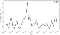
图4为采用本发明预测方法对北京2018年一月份744个时刻点的PM10浓度预测值与实际值的对比图。FIG4 is a comparison chart of the predicted value and the actual value of PM10 concentration at 744 time points in Beijing in January 2018 using the prediction method of the present invention.

图5为采用BP网络预测方法对北京2018年一月份744个时刻点的PM10浓度预测值与实际值的对比图。Figure 5 is a comparison of the predicted and actual values of PM10 concentration at 744 time points in Beijing in January 2018 using the BP network prediction method.

图6为采用LSTM网络预测方法对北京2018年一月份744个时刻点的PM10浓度预测值与实际值的对比图。Figure 6 is a comparison of the predicted and actual values of PM10 concentration at 744 time points in Beijing in January 2018 using the LSTM network prediction method.

图7为采用WaveNet网络预测方法对北京2018年一月份744个时刻点的PM10浓度预测值与实际值的对比图。Figure 7 is a comparison of the predicted and actual values of PM10 concentration at 744 time points in Beijing in January 2018 using the WaveNet network prediction method.

图8为采用改进前的TCN网络预测方法对北京2018年一月份744个时刻点的PM10浓度预测值与实际值的对比图。Figure 8 is a comparison of the predicted and actual values of PM10 concentration at 744 time points in Beijing in January 2018 using the TCN network prediction method before improvement.

图9为选定平方绝对误差(MAE)、平方绝对值百分比误差(MAPE)、平方均方误差(MSE)、均方根误差(RMSE)和决定系数(R²)五个评价指标来对本发明预测方法(用STCN表示)、BP网络预测方法(用BP表示)、LSTM网络预测方法(用LSTM表示)、WaveNet网络预测方法(用WaveNet表示)、改进前的TCN网络预测方法(用TCN表示)的预测结果进行评价的对比图。9 is a comparison chart which selects five evaluation indicators, namely, square absolute error (MAE), square absolute percentage error (MAPE), square mean square error (MSE), root mean square error (RMSE) and determination coefficient (R² ), to evaluate the prediction results of the prediction method of the present invention (expressed by STCN), the BP network prediction method (expressed by BP), the LSTM network prediction method (expressed by LSTM), the WaveNet network prediction method (expressed by WaveNet) and the TCN network prediction method before improvement (expressed by TCN).

具体实施方式DETAILED DESCRIPTION

为了更加清晰的阐述本发明的技术方案，下面结合附图及实例，对本发明进一步详细描述。本发明的实施方式及其说明仅用于解释本发明，并不作为对本发明的限定。In order to more clearly explain the technical solution of the present invention, the present invention is further described in detail below in conjunction with the accompanying drawings and examples. The embodiments of the present invention and their descriptions are only used to explain the present invention and are not intended to limit the present invention.

本发明提供一种基于改进TCN的空气污染物浓度预测方法(简称预测方法，参见图1-4)，该预测方法的具体实施步骤如下：The present invention provides an air pollutant concentration prediction method based on improved TCN (referred to as prediction method, see Figures 1-4), and the specific implementation steps of the prediction method are as follows:

步骤一：将一种空气污染物浓度历史数据时间序列按一定时间间隔选取数据点，得到训练集的原始空气污染物浓度时间序列；训练集中的时间长度不少于一年；Step 1: Select data points from the historical data time series of air pollutant concentration at a certain time interval to obtain the original air pollutant concentration time series of the training set; the time length in the training set is not less than one year;

步骤二：建立改进的TCN神经网络模型Step 2: Establish an improved TCN neural network model

2.1令训练集的原始空气污染物浓度时间序列为σ，设定TCN神经网络的输入为X_σ＝(σ₁，σ₂...σ_h)，其中，h为神经网络输入数据的维度，表示在待预测的空气污染物浓度数据点对应时刻点之前的原始空气污染物浓度序列数据点的个数(1，2...h是指按顺序选取，不指代具体时刻点)。由训练集的原始空气污染物浓度时间序列σ得到多组X_σ。TCN神经网络的输出为

表示第h+1时刻的预测数据。2.1 Let the original air pollutant concentration time series of the training set be σ, and set the input of the TCN neural network to be X_σ =(σ₁ ,σ₂ ...σ_h ), where h is the dimension of the neural network input data, which represents the number of original air pollutant concentration sequence data points before the corresponding time point of the air pollutant concentration data point to be predicted (1, 2...h means selected in order, not referring to the specific time point). Multiple groups of X_σ are obtained from the original air pollutant concentration time series σ of the training set. The output of the TCN neural network is

Represents the predicted data at the h+1th time.

2.2根据预设的神经网络输入数据的维度，将一个h维度的污染物浓度时间序列X_σ输入到TCN神经网络的一维全卷积层；一维全卷积层网络采用因果卷积，可以保证预测时刻h+1的数值只与历史时刻数据有关。2.2 According to the preset dimension of the neural network input data, an h-dimensional pollutant concentration time series_Xσ is input into the one-dimensional full convolutional layer of the TCN neural network; the one-dimensional full convolutional layer network adopts causal convolution to ensure that the value at the predicted time h+1 is only related to the historical time data.

假设卷积核f：{0，...，k-1}→R，则一个h个维度的污染物浓度时间序列X_σ中某个元素σ_t的输出为：Assuming the convolution kernel f: {0, ..., k-1} → R, the output of an element σ_t in an h-dimensional pollutant concentration time series X_σ is:

上式中，σ_t表示输入序列中的某个元素，即X_σ中第t(1≤t≤h)时刻的污染物浓度数据，σ_t-i表示卷积的方向。In the above formula,_σt represents an element in the input sequence, that is, the pollutant concentration data at the tth time (1≤t≤h) in_Xσ , and_σti represents the direction of convolution.

对一个h维度的污染物浓度时间序列X_σ中的每一个元素进行如公式(1)所示的操作，得到该X_σ的总体输出C(X_σ)。The operation shown in formula (1) is performed on each element in an h-dimensional pollutant concentration time series_Xσ to obtain the overall output C(_Xσ ) of_Xσ .

2.3构建残差收缩网络，残差收缩网络由串联的j个残差收缩网络块构成，一个残差收缩网络块包括l个残差收缩块，l个残差收缩块依次串联构成一个残差收缩网络块，每一个残差收缩块均包含一个空洞因果卷积模块和残差收缩路径模块，将空洞因果卷积模块的输入和残差收缩路径模块的输出进行跳跃连接，得到该残差收缩块的输出；第一个残差收缩块(底层)的输入为步骤2.2中的一维全卷积层的输出C(X_σ)，最后一个残差收缩块(顶层)的输入为倒数第二个残差收缩块的输出，最后一个残差收缩块的输出为残差收缩网络块的输出。2.3 Construct a residual shrinkage network. The residual shrinkage network consists of j residual shrinkage network blocks connected in series. One residual shrinkage network block includes l residual shrinkage blocks. The l residual shrinkage blocks are connected in series in sequence to form a residual shrinkage network block. Each residual shrinkage block contains a void causal convolution module and a residual shrinkage path module. The input of the void causal convolution module and the output of the residual shrinkage path module are jump-connected to obtain the output of the residual shrinkage block. The input of the first residual shrinkage block (bottom layer) is the output C(X_σ ) of the one-dimensional full convolution layer in step 2.2. The input of the last residual shrinkage block (top layer) is the output of the second to last residual shrinkage block. The output of the last residual shrinkage block is the output of the residual shrinkage network block.

空洞因果卷积模块由两组空洞因果卷积层、归一化层、激活函数Relu操作层、Dropout层按顺序由底层往上层依次衔接而成。将第一个空洞因果卷积层的输出经过归一化层、激活函数Relu操作层、Dropout层处理后的数据作为第二个空洞因果卷积层的输入，将第二个空洞因果卷积层的输出经过归一化层、激活函数Relu操作层、Dropout层处理后的数据作为该空洞因果卷积模块的输出，每一个空洞因果卷积层只包含一层空洞因果卷积网络；一个空洞因果卷积模块中的两个空洞因果卷积层的空洞因子d_i相同，每一个残差收缩块中的空洞因果卷积模块结构相同，卷积核大小都相同，不同残差收缩块的空洞因子d_i不同，d_i∈[d₁，…，d_l]，i对应第i个残差收缩块。The atrous causal convolution module is composed of two groups of atrous causal convolution layers, normalization layers, activation function Relu operation layers, and Dropout layers connected in order from the bottom layer to the top layer. The output of the first atrous causal convolution layer is processed by the normalization layer, the activation function Relu operation layer, and the Dropout layer as the input of the second atrous causal convolution layer, and the output of the second atrous causal convolution layer is processed by the normalization layer, the activation function Relu operation layer, and the Dropout layer as the output of the atrous causal convolution module. Each atrous causal convolution layer contains only one layer of atrous causal convolution network; the atrous factors d_i of the two atrous causal convolution layers in a atrous causal convolution module are the same, the atrous causal convolution modules in each residual shrinkage block have the same structure, the convolution kernel size is the same, and the atrous factors d_i of different residual shrinkage blocks are different, d_i ∈ [d₁ ,…, d_l ], i corresponds to the i-th residual shrinkage block.

对于第一个残差收缩网络块第一个残差收缩块(底层)，将步骤2.2中一个X_σ的总体输出C(X_σ)作为其空洞因果卷积模块的输入样本，首先经过第一个空洞因果卷积层，空洞因子的引入能够确保模型在不改变卷积核大小的情况下也能接受更长的输入。在空洞因果卷积层上将使用上一层t和t-d_i时刻的数据，来预测当前层t时刻的数据，若t-d_i时刻的数据在输入样本中不存在，则以0替补。那么第一个空洞因果卷积层的输出结果如下：For the first residual contraction network block, the first residual contraction block (bottom layer) uses the overall output C(X_σ ) of X_σ in step 2.2 as the input sample of its dilated causal convolution module. It first passes through the first dilated causal convolution layer. The introduction of the dilated factor ensures that the model can accept longer inputs without changing the size of the convolution kernel. The data at the previous layer at time t and td_i will be used on the dilated causal convolution layer to predict the data at time t of the current layer. If the data at time td_i does not exist in the input sample, it will be replaced by 0. Then the output of the first dilated causal convolution layer is as follows:

其中

表示X_σ中的第t-d₁时刻的污染物浓度数据经过一维全卷积层后的输出，C(σ_t)同理，d₁为第一个残差收缩块的空洞因果卷积模块的两层空洞因果卷积层的空洞因子；权重设为F(W)＝(W⁽¹⁾，W⁽²⁾)，W⁽¹⁾、W⁽²⁾是一组针对于该空洞因果卷积层卷积核的权重，W⁽¹⁾、W⁽²⁾的初始值是由网络中Glorot均匀分布初始化方法生成；

是偏移量，b的初始值为0，f表示一个非线性激活函数，在该网络中采用Relu函数，下同；in

represents the output of the pollutant concentration data at the td_1th moment in_Xσ after passing through the one-dimensional full convolution layer. Similarly, C(_σt ) is_the dilution factor of the two dilution causal convolution layers of the dilution causal convolution module of the first residual contraction block. The weight is set to F(W)=(W⁽¹⁾ , W⁽²⁾ ), where W⁽¹⁾ and W⁽²⁾ are a set of weights for the convolution kernel of the dilution causal convolution layer. The initial values of W⁽¹⁾ and W⁽²⁾ are generated by the Glorot uniform distribution initialization method in the network.

is the offset, the initial value of b is 0, f represents a nonlinear activation function, and the Relu function is used in this network, the same below;

则第二个空洞因果卷积层的输出为：Then the output of the second hole causal convolutional layer is:

为第一个空洞因果卷积层输出中的t-d₁时刻数据经归一化层、激活函数Relu操作层、Dropout层处理后得到的结果，

同理。

It is the result obtained by processing the data at time td₁ in the output of the first void causal convolutional layer through the normalization layer, the activation function Relu operation layer, and the Dropout layer.

Same reason.

将第二个空洞因果卷积层的输出经归一化层、激活函数Relu操作层、Dropout层处理后，得到第一个残差收缩块的空洞因果卷积模块的输出

对一维全卷积的输出C(X_σ)中的h个时刻的每个数据进行如公式(2)、公式(3)中的操作，得到总体输出E(X_σ)^(1，1)，以下简写为E^(1，1)。The output of the second dilated causal convolutional layer is processed by the normalization layer, the activation function Relu operation layer, and the Dropout layer to obtain the output of the dilated causal convolutional module of the first residual shrinkage block.

The operations in formula (2) and formula (3) are performed on each data at h moments in the output C(X_σ ) of the one-dimensional full convolution to obtain the overall output E(X_σ )^(1,1) , hereinafter abbreviated as E^(1,1) .

将第一个残差收缩块的空洞因果卷积模块的输出E^(1，1)作为第一个残差收缩块的残差收缩路径模块的输入，残差收缩路径模块首先对输出E^(1，1)求绝对值，经过全局均值池化(Global Average Pooling，GAP)处理后，获得一个E^(1，1)的特征值，记为A^(1，1)；将特征值记为A^(1，1)输入到残差第一全连接网络层中，然后将残差第一全连接网络层的输出批处理归一化到0-1之间，再依次经过激活函数Relu处理、残差第二全连接层和激活函数Sigmoid处理后，获得一个系数，记为α^(1，1)；令残差收缩路径模块的自适应阈值为τ，对空洞因果卷积模块的输出E^(1，1)进行软阈值化处理，得到残差收缩路径模块的输出

The output E^{(1, 1)} of the hole causal convolution module of the first residual contraction block is used as the input of the residual contraction path module of the first residual contraction block. The residual contraction path module first calculates the absolute value of the output E^{(1, 1)} , and obtains an eigenvalue of E^{(1, 1)} after global average pooling (GAP) processing, which is recorded as A^{(1, 1)} ; the eigenvalue is recorded as A^{(1, 1)} and input into the residual first fully connected network layer, and then the output of the residual first fully connected network layer is batch normalized to between 0 and 1, and then processed by the activation function Relu, the residual second fully connected layer and the activation function Sigmoid in turn to obtain a coefficient, which is recorded as α^{(1, 1)} ; the adaptive threshold of the residual contraction path module is set to τ, and the output E^{(1, 1)} of the hole causal convolution module is soft-thresholded to obtain the output of the residual contraction path module

上式中，τ＝α^(1，1)×A^(1，1)。通过软阈值化，网络将与当前输入样本任务无关的特征，置为0；将有关的特征，保留下来。In the above formula, τ = α^{(1, 1)} × A^{(1, 1)} . Through soft thresholding, the network sets the features that are irrelevant to the current input sample task to 0 and retains the relevant features.

将第一个残差收缩块的空洞因果卷积模块的输入和残差收缩路径模块的输出进行跳跃连接，得到第一个残差收缩网络块的第一个残差收缩块的输出：The input of the hole causal convolution module of the first residual contraction block and the output of the residual contraction path module are skipped to obtain the output of the first residual contraction block of the first residual contraction network block:

其中，V和e表示跳跃连接的一组权重与偏移量。残差收缩网络中的跳跃连接是为了能够保证网络性能不会因为反向传播的梯度问题而退化。Where V and e represent a set of weights and offsets of the jump connection. The jump connection in the residual shrinkage network is to ensure that the network performance will not be degraded due to the gradient problem of back propagation.

同理，对于第一个残差收缩网络块第二个残差收缩块，其输出为：Similarly, for the first residual contraction network block and the second residual contraction block, the output is:

为第一个残差收缩网络块的第二个残差收缩块的残差收缩路径模块的输出。

It is the output of the residual contraction path module of the second residual contraction block of the first residual contraction network block.

同理，对于第一个残差收缩网络块第l个残差收缩块，其输出为：Similarly, for the first residual shrinkage network block and the lth residual shrinkage block, the output is:

S^(1，l-1)为第一个残差收缩网络块第l-1个残差收缩块的输出，

为第一个残差收缩网络块第l个残差收缩块的残差收缩路径模块的输出。S^{(1, l-1)} is the output of the l-1th residual shrinkage block of the first residual shrinkage network block,

It is the output of the residual contraction path module of the lth residual contraction block of the first residual contraction network block.

若残差收缩网络块为多个，则将多个残差收缩网络块依次串联，将前一个残差收缩网络块(朝底层方向为前)输出作为后一个残差收缩网络块(朝顶层方向为后)的输入。同理，得到第二个残差收缩网络块的第一个残差收缩块的输出为：If there are multiple residual shrinkage network blocks, connect them in series, and use the output of the previous residual shrinkage network block (towards the bottom layer as the front) as the input of the next residual shrinkage network block (towards the top layer as the back). Similarly, the output of the first residual shrinkage block of the second residual shrinkage network block is:

为第二个残差收缩网络块的第一个残差收缩块的残差收缩路径模块的输出。

It is the output of the residual shrinkage path module of the first residual shrinkage block of the second residual shrinkage network block.

同理，得到第j个残差收缩网络块第l个残差收缩块的输出：Similarly, the output of the lth residual shrinkage block of the jth residual shrinkage network block is obtained:

S^(j，l-1)为第j个残差收缩网络块第l-1个残差收缩块的输出，

为第j个残差收缩网络块第l个残差收缩块的残差收缩路径模块的输出。S^{(j, l-1)} is the output of the l-1th residual shrinkage block of the jth residual shrinkage network block,

It is the output of the residual contraction path module of the lth residual contraction block of the jth residual contraction network block.

S^(j，l)即为残差收缩网络的输出。S^{(j, l)} is the output of the residual shrinkage network.

2.4将残差收缩网络块的最顶层的残差收缩块的输出S^(j，l)输入到TCN神经网络的外层的全连接层中，外层的全连接层将最顶层的残差收缩块的输出进行综合，得到最后的预测结果

其中，g表示激活函数Linear，J和c表示外层的全连接层的一组权重和偏移量。2.4 Input the output S^{(j, l)} of the top-level residual shrinkage block of the residual shrinkage network block into the outer fully connected layer of the TCN neural network. The outer fully connected layer synthesizes the output of the top-level residual shrinkage block to obtain the final prediction result.

Among them, g represents the activation function Linear, J and c represent a set of weights and offsets of the outer fully connected layer.

步骤三：对改进的TCN神经网络模型的网络参数的训练。Step 3: Training of network parameters of the improved TCN neural network model.

将由多组X_σ分别得到的预测结果与真实数据的均值平方误差MSE作为损失函数：The mean square error MSE of the predicted results obtained by multiple groups_{of Xσ} and the actual data is used as the loss function:

其中，y_i表示真实值，

表示预测值，n为预测的数据点个数；Among them,_yi represents the true value,

represents the predicted value, n is the number of predicted data points;

网络中的所有的权重参数初始值由Glorot均匀分布方法生成，偏移量初始值设为0。采用Adam优化器，使该损失函数的值减小直至迭代次数达到设定值，把最后一次迭代得到的各权重和偏移量参数的值作为最优值。The initial values of all weight parameters in the network are generated by the Glorot uniform distribution method, and the initial value of the offset is set to 0. The Adam optimizer is used to reduce the value of the loss function until the number of iterations reaches the set value, and the values of each weight and offset parameter obtained in the last iteration are taken as the optimal values.

采用Adam优化器根据损失函数对各权重和偏移量参数的值进行优化为现有技术，其优化过程为：It is an existing technology to use the Adam optimizer to optimize the values of each weight and offset parameter according to the loss function, and the optimization process is as follows:

1)参数设置1) Parameter settings

设置步长∈，默认为0.001；设置矩估计的指数衰减速率ρ₁和ρ₂，ρ₁和ρ₂在区间[0，1)内，默认分别为0.9和0.999；设置用于数值稳定的小常数δ，默认为10^-8；迭代次数为100；Set the step size ∈, the default is 0.001; set the exponential decay rates ρ₁ and ρ₂ of the moment estimate, ρ₁ and ρ₂ are in the interval [0, 1), and the default values are 0.9 and 0.999 respectively; set the small constant δ for numerical stability, the default value is 10^-8 ; the number of iterations is 100;

2)迭代计算2) Iterative calculation

(1)初始化网络中权重和偏移量参数，设为θ[θ₀，…，θ_j]，该网络中权重使用Glorot均匀分布方法生成，偏移量初始值都为0。初始化一阶和二阶矩变量s＝0，r＝0。初始化时间t＝0(1) Initialize the weight and offset parameters in the network, set to θ[θ₀ ,…,θ_j ]. The weights in the network are generated using the Glorot uniform distribution method, and the initial values of the offsets are all 0. Initialize the first-order and second-order moment variables s=0, r=0. Initialization time t=0

(2)选取训练集中的m组样本{X_σ⁽¹⁾，…，X_σ^(m)}的数据，对应目标为训练集的预测输出{Y⁽¹⁾，…Y^(m)}。(2) Select m groups of samples {X_σ⁽¹⁾ , …, X_σ^(m) } from the training set, and the corresponding target is the predicted output {Y⁽¹⁾ , …Y^(m) } of the training set.

计算梯度：

(对θ中逐元素应用操作)Compute the gradient:

(apply operation element-wise in θ)

其中，

表示X_σ⁽ⁱ⁾在网络中的预测输出，Y⁽ⁱ⁾表示真实值。in,

represents the predicted output of_Xσ⁽ⁱ⁾ in the network, and Y⁽ⁱ⁾ represents the true value.

(3)t＝t+1 (11)(3)t＝t+1 (11)

更新有偏一阶矩估计：s＝ρ₁s+(1-ρ₁)g (12)Update biased first-order moment estimate: s = ρ₁ s + (1-ρ₁ )g (12)

更新有偏二阶矩估计：r＝ρ₂r+(1-ρ₂)g⊙g (13)Update the biased second-order moment estimate: r = ρ₂ r + (1-ρ₂ ) g⊙g (13)

修正一阶矩的偏差：

Correct the deviation of the first moment:

修正二阶矩的偏差：

Correct the deviation of the second moment:

计算更新：

(对θ中逐元素应用操作) (16)Compute updates:

(apply the operation element-wise to θ) (16)

应用更新：θ＝θ+Δθ (17)Application update: θ＝θ+Δθ (17)

(4)重复步骤(2)(3)，直至迭代次数达到100，把最后一次迭代得到的各权重和偏移量参数的值作为最优值。(4) Repeat steps (2) and (3) until the number of iterations reaches 100, and take the values of each weight and offset parameter obtained in the last iteration as the optimal value.

步骤四：将步骤三中得到的各权重和偏移量参数的最优值代入到改进的TCN神经网络模型中，利用训练集的原始空气污染物浓度时间序列中的最后h个数据点，根据步骤二中的步骤2.2到步骤2.4，得到训练集的原始空气污染物浓度时间序列之后的第一个时刻点的预测污染物浓度数据；将获得的预测污染物浓度数据顺接在原始空气污染物浓度时间序列σ的末位之后并将其作为新的原始空气污染物浓度时间序列，选取新的原始空气污染物浓度时间序列最后的h个数据点，重复步骤二中的步骤2.2到步骤2.4，得到训练集的原始空气污染物浓度时间序列之后的第二个时刻点的预测污染物浓度数据；后续时刻点的预测污染物浓度参照此过程，依次获得。Step 4: Substitute the optimal values of the weights and offset parameters obtained in step 3 into the improved TCN neural network model, and use the last h data points in the original air pollutant concentration time series of the training set to obtain the predicted pollutant concentration data at the first time point after the original air pollutant concentration time series of the training set according to steps 2.2 to 2.4 in step 2; connect the obtained predicted pollutant concentration data to the end of the original air pollutant concentration time series σ and use it as the new original air pollutant concentration time series, select the last h data points of the new original air pollutant concentration time series, repeat steps 2.2 to 2.4 in step 2, and obtain the predicted pollutant concentration data at the second time point after the original air pollutant concentration time series of the training set; refer to this process to obtain the predicted pollutant concentrations at subsequent time points.

实施例1Example 1

本实施例提供一种基于改进TCN的空气污染物浓度预测方法，该方法的具体步骤如下：This embodiment provides an air pollutant concentration prediction method based on improved TCN, and the specific steps of the method are as follows:

步骤一：选用北京的PM10浓度历史数据时间序列，将2016-2017两年的PM10浓度历史数据时间序列按每间隔1h选取浓度数据点，得到训练集的原始PM10浓度时间序列；Step 1: Select the PM10 concentration historical data time series of Beijing, select concentration data points at intervals of 1 hour from the PM10 concentration historical data time series of 2016-2017, and obtain the original PM10 concentration time series of the training set;

步骤二：建立改进的TCN神经网络模型Step 2: Establish an improved TCN neural network model

2.1令训练集的原始PM10浓度时间序列为σ，设定TCN神经网络的输入为X_σ＝(σ₁，σ₁，σ₂…σ₆)，输出为

表示第7时刻的预测PM10浓度数据。神经网络输入数据的维度为6，表示在待预测的PM10浓度数据点对应时刻点之前的原始PM10浓度时间序列数据点的个数。由训练集的原始PM10浓度时间序列σ得到多组X_σ。2.1 Let the original PM10 concentration time series of the training set be σ, set the input of the TCN neural network to X_σ = (σ₁ , σ₁ , σ₂ …σ₆ ), and the output to be

Represents the predicted PM10 concentration data at the 7th moment. The dimension of the neural network input data is 6, which represents the number of original PM10 concentration time series data points before the corresponding time point of the PM10 concentration data point to be predicted. Multiple groups of X_σ are obtained from the original PM10 concentration time series σ of the training set.

2.2根据预设的神经网络输入数据的维度，将一个6个维度的PM10浓度时间序列X_σ输入到TCN神经网络的一维全卷积层；一维全卷积层网络采用因果卷积，可以保证预测时刻7的数值只与历史时刻数据有关。2.2 According to the preset dimension of the neural network input data, a 6-dimensional PM10 concentration time series_Xσ is input into the one-dimensional full convolution layer of the TCN neural network; the one-dimensional full convolution layer network adopts causal convolution, which can ensure that the value of the predicted time 7 is only related to the historical time data.

假设卷积核f：{0，...，k-1}→R，则一个6个维度的PM10浓度时间序列X_σ中某个元素σ_t的输出为：Assuming the convolution kernel f: {0, ..., k-1} → R, the output of an element σ_t in a 6-dimensional PM10 concentration time series X_σ is:

上式中，σ_t表示输入序列中的某个元素，即X_σ中第t(1≤t≤6)时刻的PM10浓度数据，σ_t-i卷积的方向。In the above formula,_σt represents an element in the input sequence, that is, the PM10 concentration data at the tth time (1≤t≤6) in_Xσ , and_σti is the direction of convolution.

对一个6个维度的PM10浓度时间序列X_σ中的每一个元素进行如公式(1)所示的操作，得到该X_σ的总体输出C(X_σ)。The operation shown in formula (1) is performed on each element of a 6-dimensional PM10 concentration time series_Xσ to obtain the overall output C(_Xσ ) of_Xσ .

2.3构建残差收缩网络，残差收缩网络由两个残差收缩网络块串联构成，每一个残差收缩网络块包括3个残差收缩块，3个残差收缩块依次串联，每一个残差收缩块均包含一个空洞因果卷积模块和残差收缩路径模块，将空洞因果卷积模块的输入和残差收缩路径模块的输出进行跳跃连接，得到该残差收缩块的输出；第一个残差收缩块(底层)的输入为步骤2.2中的一维全卷积层的输出C(X_σ)，最后一个残差收缩块(顶层)的输入为倒数第二个残差收缩块的输出，最后一个残差收缩块的输出为残差收缩网络块的输出。空洞因果卷积模块由两组空洞因果卷积层、归一化层、激活函数Relu操作层、Dropout层按顺序由底层往上层依次衔接而成。将第一个空洞因果卷积层的输出经过归一化层、激活函数Relu操作层、Dropout层处理后的数据作为第二个空洞因果卷积层的输入，将第二个空洞因果卷积层的输出经过归一化层、激活函数Relu操作层、Dropout层处理后的数据作为该空洞因果卷积模块的输出。归一化层均采用(0，1)标准化，Dropout层的丢弃率都为0.05。2.3 Construct a residual shrinkage network. The residual shrinkage network is composed of two residual shrinkage network blocks connected in series. Each residual shrinkage network block includes three residual shrinkage blocks, which are connected in series in sequence. Each residual shrinkage block contains a void causal convolution module and a residual shrinkage path module. The input of the void causal convolution module and the output of the residual shrinkage path module are jump-connected to obtain the output of the residual shrinkage block. The input of the first residual shrinkage block (bottom layer) is the output C(X_σ ) of the one-dimensional full convolution layer in step 2.2, and the input of the last residual shrinkage block (top layer) is the output of the second-to-last residual shrinkage block. The output of the last residual shrinkage block is the output of the residual shrinkage network block. The void causal convolution module is composed of two groups of void causal convolution layers, normalization layers, activation function Relu operation layers, and Dropout layers, which are connected in sequence from the bottom layer to the top layer. The output of the first atrous causal convolutional layer is processed by the normalization layer, the activation function Relu operation layer, and the Dropout layer as the input of the second atrous causal convolutional layer, and the output of the second atrous causal convolutional layer is processed by the normalization layer, the activation function Relu operation layer, and the Dropout layer as the output of the atrous causal convolutional module. The normalization layer is standardized by (0, 1), and the dropout rate of the Dropout layer is 0.05.

两个残差收缩网络块结构相同，每一个残差收缩网络块的3个残差收缩块中的空洞因果卷积模块的空洞因子d_i∈[1，2，4]，权重F(W)＝(W⁽¹⁾，W⁽²⁾)的初始值在网络由Glorot均匀分布方法初始化。

是偏移量，在网络中初始值设为0，f表示一个非线性激活函数，在该网络中采用ReLU函数，那么第一个残差收缩网络块的第一个残差收缩块中的空洞因果卷积模块中第一层空洞因果卷积层的输出为：The two residual shrinkage network blocks have the same structure. The void factors d_i ∈ [1, 2, 4] of the void causal convolution modules in the three residual shrinkage blocks of each residual shrinkage network block, and the initial values of the weights F(W) = (W⁽¹⁾ , W⁽²⁾ ) are initialized in the network by the Glorot uniform distribution method.

is the offset, the initial value is set to 0 in the network, f represents a nonlinear activation function, and the ReLU function is used in the network. Then the output of the first hole causal convolution layer in the hole causal convolution module in the first residual contraction block of the first residual contraction network block is:

其中

表示X_σ中的第t-1时刻的PM10浓度数据经过一维全卷积层后的输出，C(σ_t)同理，空洞因子为1；in

represents the output of the PM10 concentration data at the t-1th moment in_Xσ after passing through the one-dimensional full convolutional layer. Similarly, C(_σt ) has a void factor of 1.

则第二个空洞因果卷积层的输出为：Then the output of the second hole causal convolutional layer is:

为第一个空洞因果卷积层输出中的t-1时刻数据经归一化层、激活函数Relu操作层、Dropout层处理后得到的结果，

同理。

It is the result obtained after the t-1 time data in the output of the first hole causal convolution layer is processed by the normalization layer, the activation function Relu operation layer, and the Dropout layer.

Same reason.

将第二个空洞因果卷积层的输出经归一化层、激活函数Relu操作层、Dropout层处理后，得到第一个残差收缩块的空洞因果卷积模块的输出

对一维全卷积的输出C(X_σ)中的6个时刻的每个数据进行如公式(2)、公式(3)中的操作，得到总体输出E(X_σ)^(1，1)，以下简写为E^(1，1)。The output of the second dilated causal convolutional layer is processed by the normalization layer, the activation function Relu operation layer, and the Dropout layer to obtain the output of the dilated causal convolutional module of the first residual shrinkage block.

The operations in formula (2) and formula (3) are performed on each of the six data points in the output C(X_σ ) of the one-dimensional full convolution to obtain the overall output E(X_σ )^{(1, 1)} , which is abbreviated as E^{(1, 1)} below.

将第一个残差收缩块的空洞因果卷积模块的输出E^(1，1)作为第一个残差收缩块的残差收缩路径模块的输入，残差收缩路径模块首先对输出E^(1，1)求绝对值，经过全局均值池化(Global Average Pooling，GAP)处理后，获得一个E^(1，1)的特征值，记为A^(1，1)；将特征值记为A^(1，1)输入到残差第一全连接网络层中，然后将残差第一全连接网络层的输出批处理归一化到0-1之间，再依次经过激活函数Relu处理、残差第二全连接层和激活函数Sigmoid处理后，获得一个系数，记为α^(1，1)；令残差收缩路径模块的自适应阈值为τ，对空洞因果卷积模块的输出E^(1，1)进行软阈值化处理，得到残差收缩路径模块的输出

The output E^{(1, 1)} of the hole causal convolution module of the first residual contraction block is used as the input of the residual contraction path module of the first residual contraction block. The residual contraction path module first calculates the absolute value of the output E^{(1, 1)} , and obtains an eigenvalue of E^{(1, 1)} after global average pooling (GAP) processing, which is recorded as A^{(1, 1)} ; the eigenvalue is recorded as A^{(1, 1)} and input into the residual first fully connected network layer, and then the output of the residual first fully connected network layer is batch normalized to between 0 and 1, and then processed by the activation function Relu, the residual second fully connected layer and the activation function Sigmoid in turn to obtain a coefficient, which is recorded as α^{(1, 1)} ; the adaptive threshold of the residual contraction path module is set to τ, and the output E^{(1, 1)} of the hole causal convolution module is soft-thresholded to obtain the output of the residual contraction path module

上式中，τ＝α^(1，1)×A^(1，1)。通过软阈值化，网络将与当前输入样本任务无关的特征，置为0；将有关的特征，保留下来。In the above formula, τ = α^{(1, 1)} × A^{(1, 1)} . Through soft thresholding, the network sets the features that are irrelevant to the current input sample task to 0 and retains the relevant features.

将第一个残差收缩块的空洞因果卷积模块的输入和残差收缩路径模块的输出进行跳跃连接，得到第一个残差收缩网络块的第一个残差收缩块的输出：The input of the hole causal convolution module of the first residual contraction block and the output of the residual contraction path module are skipped to obtain the output of the first residual contraction block of the first residual contraction network block:

其中，V和e表示跳跃连接的一组权重与偏移量，设置为1和0。残差收缩网络中的跳跃连接是为了能够保证网络性能不会因为反向传播的梯度问题而退化。Among them, V and e represent a set of weights and offsets of the jump connection, which are set to 1 and 0. The jump connection in the residual shrinkage network is to ensure that the network performance will not be degraded due to the gradient problem of back propagation.

第一个残差收缩网络块的第二个残差收缩块中的第一个空洞因果卷积层的输出为：The output of the first atrous causal convolutional layer in the second residual contraction block of the first residual contraction network block is:

其中

表示第一个残差收缩网络块的第二个残差收缩块输出中的t-2时刻数据，

同理，空洞因子为2。in

Represents the t-2 time data in the output of the second residual shrinkage block of the first residual shrinkage network block,

Similarly, the void factor is 2.

第一个残差收缩网络块的第二个残差收缩块中的第二个空洞因果卷积层的输出为：The output of the second atrous causal convolutional layer in the second residual contraction block of the first residual contraction network block is:

为第二个残差收缩块中第一个空洞因果卷积层输出中的t-2时刻数据经归一化层、激活函数Relu操作层、Dropout层处理后得到的结果，

同理。

It is the result obtained by processing the t-2 time data in the output of the first hole causal convolution layer in the second residual contraction block through the normalization layer, the activation function Relu operation layer, and the Dropout layer.

Same reason.

同理，第一个残差收缩网络块的第二个残差收缩块的输出为：Similarly, the output of the second residual shrinkage block of the first residual shrinkage network block is:

为第一个残差收缩网络块的第二个残差收缩块的残差收缩路径模块的输出。

It is the output of the residual contraction path module of the second residual contraction block of the first residual contraction network block.

同理，第一个残差收缩网络块的第三个残差收缩块的输出为：Similarly, the output of the third residual shrinkage block of the first residual shrinkage network block is:

为第一个残差收缩网络块的第三个残差收缩块的残差收缩路径模块的输出。

It is the output of the residual contraction path module of the third residual contraction block of the first residual contraction network block.

同理，第二个残差收缩网络块的第一个残差收缩块的输出为：Similarly, the output of the first residual shrinkage block of the second residual shrinkage network block is:

为第二个残差收缩网络块的第一个残差收缩块的残差收缩路径模块的输出。

It is the output of the residual shrinkage path module of the first residual shrinkage block of the second residual shrinkage network block.

第二个残差收缩网络块的第二个残差收缩块的输出为：The output of the second residual shrinkage block of the second residual shrinkage network block is:

为第二个残差收缩网络块的第二个残差收缩块的残差收缩路径模块的输出。

It is the output of the residual contraction path module of the second residual contraction block of the second residual contraction network block.

第二个残差收缩网络块的第三个残差收缩块的输出为：The output of the third residual shrinkage block of the second residual shrinkage network block is:

为第二个残差收缩网络块的第三个残差收缩块的残差收缩路径模块的输出。

It is the output of the residual contraction path module of the third residual contraction block of the second residual contraction network block.

S^(2，3)即为残差收缩网络的输出。S^{(2, 3)} is the output of the residual shrinkage network.

2.4将残差收缩网络的输出S^(2，3)输入到TCN神经网络的外层的全连接层中，外层的全连接层将最顶层的残差收缩块的输出进行综合，得到最后的预测结果

其中，g表示激活函数Linear，J和c表示外层的全连接层的一组权重和偏移量。2.4 Input the output S^{(2, 3)} of the residual shrinkage network into the outer fully connected layer of the TCN neural network. The outer fully connected layer integrates the output of the topmost residual shrinkage block to obtain the final prediction result.

Among them, g represents the activation function Linear, J and c represent a set of weights and offsets of the outer fully connected layer.

步骤三：对改进的TCN神经网络模型的网络参数的训练。Step 3: Training of network parameters of the improved TCN neural network model.

将由多组X_σ分别得到的预测结果与真实数据的均值平方误差MSE作为损失函数：The mean square error MSE of the predicted results obtained by multiple groups_{of Xσ} and the actual data is used as the loss function:

其中，y_i表示真实值，

表示预测值，n为预测的数据点个数；Among them,_yi represents the true value,

represents the predicted value, n is the number of predicted data points;

网络中的所有的权重参数初始值由Glorot均匀分布方法生成，偏移量初始值设为0。采用Adam优化器，使该损失函数的值减小直至迭代次数达到100，把最后一次迭代得到的各权重和偏移量参数的值作为最优值。The initial values of all weight parameters in the network are generated by the Glorot uniform distribution method, and the initial value of the offset is set to 0. The Adam optimizer is used to reduce the value of the loss function until the number of iterations reaches 100, and the values of each weight and offset parameter obtained in the last iteration are taken as the optimal values.

步骤四：将步骤三中得到的各权重和偏移量参数的最优值代入到改进的TCN神经网络模型中，利用训练集的原始PM10浓度时间序列中的最后6个数据点，根据步骤二中的步骤2.2到步骤2.4，得到2018年一月份的第一天的第一个时刻点的预测PM10浓度数据；将获得的预测PM10浓度数据顺接在原始PM10浓度时间序列σ的末位之后并将其作为新的原始PM10浓度时间序列，选取新的原始PM10浓度时间序列最后的6个数据点，重复步骤二中的步骤2.2到步骤2.4，得到2018年一月份的第一天的第二个时刻点的预测PM10浓度数据；后续时刻点的预测PM10浓度参照此过程，依次获得2018年一月份的744个时刻点的预测PM10浓度数据。Step 4: Substitute the optimal values of the weights and offset parameters obtained in step 3 into the improved TCN neural network model, and use the last 6 data points in the original PM10 concentration time series of the training set to obtain the predicted PM10 concentration data at the first time point of the first day of January 2018 according to steps 2.2 to 2.4 in step 2; connect the obtained predicted PM10 concentration data to the end of the original PM10 concentration time series σ and use it as the new original PM10 concentration time series, select the last 6 data points of the new original PM10 concentration time series, repeat steps 2.2 to 2.4 in step 2, and obtain the predicted PM10 concentration data at the second time point of the first day of January 2018; refer to this process for the predicted PM10 concentrations at subsequent time points, and obtain the predicted PM10 concentration data for 744 time points in January 2018 in turn.

根据本发明预测方法，得到2018年一月份744个时刻点的PM10浓度预测值；将2018年一月份744个时刻点的PM10浓度的实际值作为测试集；2018年一月份的预测的744个时刻点的PM10浓度数据

与测试集中的实际数据y_i进行对比，如图4所示(本发明预测方法所得预测数据用STCN表示，实际数据y_i用Actual表示，下同)；According to the prediction method of the present invention, the predicted values of PM10 concentration at 744 time points in January 2018 are obtained; the actual values of PM10 concentration at 744 time points in January 2018 are used as the test set; the PM10 concentration data of the predicted 744 time points in January 2018 are

Compare with the actual data_yi in the test set, as shown in FIG4 (the predicted data obtained by the prediction method of the present invention is represented by STCN, and the actual data_yi is represented by Actual, the same below);

对同样的训练集和测试集，采用BP网络预测方法(用BP表示)、LSTM网络预测方法(用LSTM表示)、WaveNet网络预测方法(用WaveNet表示)、改进前的TCN网络预测方法(用TCN表示)分别进行预测，该四种预测方法的结果与测试集中的实际数据y_i的对比图见图5-8。For the same training set and test set, the BP network prediction method (represented by BP), LSTM network prediction method (represented by LSTM), WaveNet network prediction method (represented by WaveNet), and TCN network prediction method before improvement (represented by TCN) are used for prediction respectively. The comparison between the results of the four prediction methods and the actual data y_i in the test set is shown in Figures 5-8.

选定平方绝对误差(MAE)、平方绝对值百分比误差(MAPE)、平方均方误差(MSE)、均方根误差(RMSE)和决定系数(R²)五个评价指标来对本发明预测方法(用STCN表示)、BP网络预测方法(用BP表示)、LSTM网络预测方法(用LSTM表示)、WaveNet网络预测方法(用WaveNet表示)、改进前的TCN网络预测方法(用TCN表示)的预测结果进行评价。具体计算公式为：The five evaluation indicators of square absolute error (MAE), square absolute percentage error (MAPE), square mean square error (MSE), root mean square error (RMSE) and determination coefficient (R² ) are selected to evaluate the prediction results of the prediction method of the present invention (expressed as STCN), BP network prediction method (expressed as BP), LSTM network prediction method (expressed as LSTM), WaveNet network prediction method (expressed as WaveNet), and TCN network prediction method before improvement (expressed as TCN). The specific calculation formula is:

数值越小说明预测越准确；

The smaller the value, the more accurate the prediction;

数值越小说明预测越准确；

The smaller the value, the more accurate the prediction;

数值越小说明预测越准确；

The smaller the value, the more accurate the prediction;

数值越小说明预测越准确；

The smaller the value, the more accurate the prediction;

数值越大说明预测越准确；

The larger the value, the more accurate the prediction;

其中，y_i表示真实值，

表示预测值，

为真实值y_i的平均值。Among them,_yi represents the true value,

represents the predicted value,

is the average value of the true value_yi .

五种预测方法的五种评价指标的对比如图9所示，结果显示，本发明预测方法所得结果更接近实测PM10浓度，通过与其它神经网络预测方法对比，本发明预测方法所得到的预测结果的稳定性更好，准确性更高。A comparison of five evaluation indicators of five prediction methods is shown in FIG9 . The results show that the result obtained by the prediction method of the present invention is closer to the measured PM10 concentration. By comparing with other neural network prediction methods, the prediction result obtained by the prediction method of the present invention has better stability and higher accuracy.

本发明未述及之处适用于现有技术。Any matters not described in the present invention are applicable to the prior art.

Claims (8)

Translated fromChinese

1.一种基于改进TCN的空气污染物浓度预测方法，其特征在于，该预测方法的具体实施步骤如下：1. A method for predicting air pollutant concentration based on improved TCN, characterized in that the specific implementation steps of the prediction method are as follows:步骤一：将一种空气污染物浓度历史数据时间序列按一定时间间隔选取数据点，得到训练集的原始空气污染物浓度时间序列；训练集中的时间长度不少于一年；Step 1: Select data points from the historical data time series of air pollutant concentration at a certain time interval to obtain the original air pollutant concentration time series of the training set; the time length in the training set is not less than one year;步骤二：建立改进的TCN神经网络模型Step 2: Establish an improved TCN neural network model2.1令训练集的原始空气污染物浓度时间序列为σ，设定TCN神经网络的输入为X_σ＝(σ₁,σ₂…σ_h),其中，h为神经网络输入数据的维度，表示在待预测的空气污染物浓度数据点对应时刻点之前的原始空气污染物浓度序列数据点的个数；由训练集的原始空气污染物浓度时间序列σ得到多组X_σ；TCN神经网络的输出为

表示第h+1时刻的预测数据；2.1 Let the original air pollutant concentration time series of the training set be σ, and set the input of the TCN neural network to be X_σ =(σ₁ ,σ₂ …σ_h ), where h is the dimension of the neural network input data, indicating the number of original air pollutant concentration sequence data points before the corresponding time point of the air pollutant concentration data point to be predicted; multiple groups of X_σ are obtained from the original air pollutant concentration time series σ of the training set; the output of the TCN neural network is

Represents the predicted data at the h+1th moment;2.2根据预设的神经网络输入数据的维度，将一个h维度的污染物浓度时间序列X_σ输入到TCN神经网络的一维全卷积层；一维全卷积层网络采用因果卷积；2.2 According to the dimension of the preset neural network input data, an h-dimensional pollutant concentration time series_Xσ is input into the one-dimensional full convolution layer of the TCN neural network; the one-dimensional full convolution layer network adopts causal convolution;假设卷积核f:{0,…,k-1}→R，则一个h个维度的污染物浓度时间序列X_σ中某个元素σ_t的输出为：Assuming the convolution kernel f:{0,…,k-1}→R, the output of an element_σt in an h-dimensional pollutant concentration time series_Xσ is:

上式中，σ_t表示输入序列中的某个元素，即X_σ中第t时刻的污染物浓度数据，σ_t-i表示卷积的方向；In the above formula, σ_t represents an element in the input sequence, that is, the pollutant concentration data at the tth time in X_σ , and σ_ti represents the direction of convolution;对一个h维度的污染物浓度时间序列X_σ中的每一个元素进行如公式(1)所示的操作，得到该X_σ的总体输出C(X_σ)；Perform the operation shown in formula (1) on each element of an h-dimensional pollutant concentration time series X_σ to obtain the overall output C(X_σ ) of X_σ ;2.3构建残差收缩网络，残差收缩网络由串联的j个残差收缩网络块构成，一个残差收缩网络块包括l个残差收缩块，l个残差收缩块依次串联构成一个残差收缩网络块，每一个残差收缩块均包含一个空洞因果卷积模块和残差收缩路径模块，将空洞因果卷积模块的输入和残差收缩路径模块的输出进行跳跃连接，得到该残差收缩块的输出；第一个残差收缩块的输入为步骤2.2中的一维全卷积层的输出C(X_σ)，最后一个残差收缩块的输入为倒数第二个残差收缩块的输出，最后一个残差收缩块的输出为残差收缩网络块的输出；2.3 Construct a residual contraction network. The residual contraction network consists of j residual contraction network blocks connected in series. One residual contraction network block includes l residual contraction blocks. The l residual contraction blocks are connected in series in sequence to form a residual contraction network block. Each residual contraction block includes a void causal convolution module and a residual contraction path module. The input of the void causal convolution module and the output of the residual contraction path module are jump-connected to obtain the output of the residual contraction block. The input of the first residual contraction block is the output C(X_σ ) of the one-dimensional full convolution layer in step 2.2. The input of the last residual contraction block is the output of the second to last residual contraction block. The output of the last residual contraction block is the output of the residual contraction network block.空洞因果卷积模块由两组空洞因果卷积层、归一化层、激活函数Relu操作层、Dropout层按顺序由底层往上层依次衔接而成；将第一个空洞因果卷积层的输出经过归一化层、激活函数Relu操作层、Dropout层处理后的数据作为第二个空洞因果卷积层的输入，将第二个空洞因果卷积层的输出经过归一化层、激活函数Relu操作层、Dropout层处理后的数据作为该空洞因果卷积模块的输出，每一个空洞因果卷积层只包含一层空洞因果卷积网络；一个空洞因果卷积模块中的两个空洞因果卷积层的空洞因子d_i相同，每一个残差收缩块中的空洞因果卷积模块结构相同，卷积核大小都相同，不同残差收缩块的空洞因子d_i不同，d_i∈[d₁，…，d_l]，i对应第i个残差收缩块；The atrous causal convolution module is composed of two groups of atrous causal convolution layers, a normalization layer, an activation function Relu operation layer, and a Dropout layer, which are connected in sequence from the bottom layer to the upper layer; the output of the first atrous causal convolution layer is processed by the normalization layer, the activation function Relu operation layer, and the Dropout layer as the input of the second atrous causal convolution layer, and the output of the second atrous causal convolution layer is processed by the normalization layer, the activation function Relu operation layer, and the Dropout layer as the output of the atrous causal convolution module, and each atrous causal convolution layer contains only one layer of atrous causal convolution network; the atrous factors d_i of the two atrous causal convolution layers in a atrous causal convolution module are the same, the atrous causal convolution modules in each residual shrinkage block have the same structure, the convolution kernel size is the same, and the atrous factors d_i of different residual shrinkage blocks are different, d_i ∈ [d₁ , … , d_l ], i corresponds to the i-th residual shrinkage block;对于第一个残差收缩网络块第一个残差收缩块，将步骤2.2中一个X_σ的总体输出C(X_σ)作为其空洞因果卷积模块的输入样本，首先经过第一个空洞因果卷积层；在空洞因果卷积层上将使用上一层t和t-d_i时刻的数据，来预测当前层t时刻的数据，若t-d_i时刻的数据在输入样本中不存在，则以0替补；那么第一个空洞因果卷积层的输出结果如下：For the first residual contraction network block, the overall output C(X_σ ) of X_σ in step 2.2 is used as the input sample of its void causal convolution module, and first passes through the first void causal convolution layer; the void causal convolution layer will use the data of the previous layer at time t and td_i to predict the data of the current layer at time t. If the data at time td_i does not exist in the input sample, it will be replaced by 0; then the output result of the first void causal convolution layer is as follows:

其中

表示X_σ中的第t-d₁时刻的污染物浓度数据经过一维全卷积层后的输出，C(σ_t)同理，d₁为第一个残差收缩块的空洞因果卷积模块的两层空洞因果卷积层的空洞因子；权重设为F(W)＝(W⁽¹⁾,W⁽²⁾)，W⁽¹⁾、W⁽²⁾是一组针对于该空洞因果卷积层卷积核的权重，W⁽¹⁾、W⁽²⁾的初始值是由Glorot均匀分布初始化方法生成；

是偏移量，b的初始值为0，f表示一个非线性激活函数，在该网络中采用Relu函数，下同；in

represents the output of the pollutant concentration data at the td_1th moment in_Xσ after passing through the one-dimensional full convolution layer. Similarly, C(_σt ) is d1, and_d1 is the dilution factor of the two dilution causal convolution layers of the dilution causal convolution module of the first residual contraction block. The weight is set to F(W) = (W⁽¹⁾ , W⁽²⁾ ), where W⁽¹⁾ and W⁽²⁾ are a set of weights for the convolution kernel of the dilution causal convolution layer. The initial values of W⁽¹⁾ and W⁽²⁾ are generated by the Glorot uniform distribution initialization method.

is the offset, the initial value of b is 0, f represents a nonlinear activation function, and the Relu function is used in this network, the same below;则第二个空洞因果卷积层的输出为：Then the output of the second hole causal convolutional layer is:

为第一个空洞因果卷积层输出中的t-d₁时刻数据经归一化层、激活函数Relu操作层、Dropout层处理后得到的结果，

同理；

It is the result obtained by processing the data at time td₁ in the output of the first void causal convolutional layer through the normalization layer, the activation function Relu operation layer, and the Dropout layer.

Similarly;将第二个空洞因果卷积层的输出经归一化层、激活函数Relu操作层、Dropout层处理后，得到第一个残差收缩块的空洞因果卷积模块的输出

对一维全卷积的输出C(X_σ)中的h个时刻的每个数据进行如公式(2)、公式(3)中的操作，得到总体输出E(X_σ)^(1,1),以下简写为E^(1,1)；The output of the second dilated causal convolutional layer is processed by the normalization layer, the activation function Relu operation layer, and the Dropout layer to obtain the output of the dilated causal convolutional module of the first residual shrinkage block.

Perform the operations in formula (2) and formula (3) on each data at h moments in the output C(X_σ ) of the one-dimensional full convolution to obtain the overall output E(X_σ )^(1,1) , hereinafter abbreviated as E^(1,1) ;将第一个残差收缩块的空洞因果卷积模块的输出E^(1,1)作为第一个残差收缩块的残差收缩路径模块的输入，残差收缩路径模块首先对输出E^(1,1)求绝对值，经过全局均值池化处理后，获得一个E^(1,1)的特征值，记为A^(1,1)；将特征值记为A^(1,1)输入到残差第一全连接网络层中，然后将残差第一全连接网络层的输出批处理归一化到0-1之间，再依次经过激活函数Relu处理、残差第二全连接层和激活函数Sigmoid处理后，获得一个系数，记为α^(1,1)；令残差收缩路径模块的自适应阈值为τ，对空洞因果卷积模块的输出E^(1,1)进行软阈值化处理，得到残差收缩路径模块的输出

The output E^(1,1) of the hole causal convolution module of the first residual shrinkage block is used as the input of the residual shrinkage path module of the first residual shrinkage block. The residual shrinkage path module first calculates the absolute value of the output E^(1,1) , and obtains an eigenvalue of E^(1,1) after global mean pooling, denoted as A^(1,1) ; the eigenvalue is denoted as A^(1,1) and input into the residual first fully connected network layer, and then the output of the residual first fully connected network layer is batch normalized to between 0 and 1, and then processed by the activation function Relu, the residual second fully connected layer and the activation function Sigmoid in turn to obtain a coefficient, denoted as α^(1,1) ; the adaptive threshold of the residual shrinkage path module is set to τ, and the output E^(1,1) of the hole causal convolution module is soft-thresholded to obtain the output of the residual shrinkage path module

上式中，τ＝α^(1,1)×A^(1,1)；In the above formula, τ=α^(1,1) ×A^(1,1) ;将第一个残差收缩块的空洞因果卷积模块的输入和残差收缩路径模块的输出进行跳跃连接，得到第一个残差收缩网络块的第一个残差收缩块的输出：The input of the hole causal convolution module of the first residual contraction block and the output of the residual contraction path module are skipped to obtain the output of the first residual contraction block of the first residual contraction network block:

其中，V和e表示跳跃连接的一组权重与偏移量；Among them, V and e represent a set of weights and offsets of the jump connection;同理，对于第一个残差收缩网络块第二个残差收缩块，其输出为：Similarly, for the first residual shrinkage network block and the second residual shrinkage block, the output is:

为第一个残差收缩网络块的第二个残差收缩块的残差收缩路径模块的输出；

The output of the residual contraction path module of the second residual contraction block of the first residual contraction network block;同理，对于第一个残差收缩网络块第l个残差收缩块，其输出为：Similarly, for the first residual shrinkage network block and the lth residual shrinkage block, the output is:

S^(1,l-1)为第一个残差收缩网络块第l-1个残差收缩块的输出，

为第一个残差收缩网络块第l个残差收缩块的残差收缩路径模块的输出；S^{(1, l-1)} is the output of the l-1th residual shrinkage block of the first residual shrinkage network block,

The output of the residual contraction path module of the lth residual contraction block of the first residual contraction network block;若残差收缩网络块为多个，则将多个残差收缩网络块依次串联，将前一个残差收缩网络块输出作为后一个残差收缩网络块的输入；同理，得到第二个残差收缩网络块的第一个残差收缩块的输出为：If there are multiple residual shrinkage network blocks, the multiple residual shrinkage network blocks are connected in series, and the output of the previous residual shrinkage network block is used as the input of the next residual shrinkage network block; similarly, the output of the first residual shrinkage block of the second residual shrinkage network block is:

为第二个残差收缩网络块的第一个残差收缩块的残差收缩路径模块的输出；

The output of the residual shrinkage path module of the first residual shrinkage block of the second residual shrinkage network block;同理，得到第j个残差收缩网络块第l个残差收缩块的输出：Similarly, the output of the lth residual shrinkage block of the jth residual shrinkage network block is obtained:

S^(j,l-1)为第j个残差收缩网络块第l-1个残差收缩块的输出，

为第j个残差收缩网络块第l个残差收缩块的残差收缩路径模块的输出；S^{(j, l-1)} is the output of the l-1th residual shrinkage block of the jth residual shrinkage network block,

is the output of the residual contraction path module of the lth residual contraction block of the jth residual contraction network block;S^(j,l)即为残差收缩网络的输出；S^(j,l) is the output of the residual shrinkage network;2.4将残差收缩网络块的最顶层的残差收缩块的输出S^(j,l)输入到TCN神经网络的外层的全连接层中，外层的全连接层将最顶层的残差收缩块的输出进行综合，得到最后的预测结果

其中，g表示激活函数Linear，J和c表示外层的全连接层的一组权重和偏移量；2.4 Input the output S^{(j, l)} of the top-level residual shrinkage block of the residual shrinkage network block into the outer fully connected layer of the TCN neural network. The outer fully connected layer synthesizes the output of the top-level residual shrinkage block to obtain the final prediction result.

Among them, g represents the activation function Linear, J and c represent a set of weights and offsets of the outer fully connected layer;步骤三：对改进的TCN神经网络模型的网络参数的训练；Step 3: Training the network parameters of the improved TCN neural network model;将由多组X_σ分别得到的预测结果与真实数据的均值平方误差MSE作为损失函数：The mean square error MSE of the predicted results obtained by multiple groups_{of Xσ} and the actual data is used as the loss function:

其中，y_i表示真实值，

表示预测值，n为预测的数据点个数；Among them,_yi represents the true value,

represents the predicted value, n is the number of predicted data points;网络中的所有的权重参数初始值由Glorot均匀分布方法生成，偏移量初始值设为0；采用Adam优化器，使该损失函数的值减小直至迭代次数达到设定值，把最后一次迭代得到的各权重和偏移量参数的值作为最优值；The initial values of all weight parameters in the network are generated by the Glorot uniform distribution method, and the initial value of the offset is set to 0. The Adam optimizer is used to reduce the value of the loss function until the number of iterations reaches the set value, and the values of each weight and offset parameter obtained in the last iteration are taken as the optimal values.步骤四：将步骤三中得到的各权重和偏移量参数的最优值代入到改进的TCN神经网络模型中，利用训练集的原始空气污染物浓度时间序列中的最后h个数据点，根据步骤二中的步骤2.2到步骤2.4，得到训练集的原始空气污染物浓度时间序列之后的第一个时刻点的预测污染物浓度数据；将获得的预测污染物浓度数据顺接在原始空气污染物浓度时间序列σ的末位之后并将其作为新的原始空气污染物浓度时间序列，选取新的原始空气污染物浓度时间序列最后的h个数据点，重复步骤二中的步骤2.2到步骤2.4，得到训练集的原始空气污染物浓度时间序列之后的第二个时刻点的预测污染物浓度数据；后续时刻点的预测污染物浓度参照此过程，依次获得。Step 4: Substitute the optimal values of the weights and offset parameters obtained in step 3 into the improved TCN neural network model, and use the last h data points in the original air pollutant concentration time series of the training set to obtain the predicted pollutant concentration data at the first time point after the original air pollutant concentration time series of the training set according to steps 2.2 to 2.4 in step 2; connect the obtained predicted pollutant concentration data to the end of the original air pollutant concentration time series σ and use it as the new original air pollutant concentration time series, select the last h data points of the new original air pollutant concentration time series, repeat steps 2.2 to 2.4 in step 2, and obtain the predicted pollutant concentration data at the second time point after the original air pollutant concentration time series of the training set; refer to this process to obtain the predicted pollutant concentrations at subsequent time points.2.根据权利要求1所述的一种基于改进TCN的空气污染物浓度预测方法，其特征在于，训练集中的时间长度为两年，数据点之间的时间间隔为1h。2. The method for predicting air pollutant concentration based on improved TCN according to claim 1 is characterized in that the time length in the training set is two years and the time interval between data points is 1 hour.3.根据权利要求1所述的一种基于改进TCN的空气污染物浓度预测方法，其特征在于，设定TCN神经网络的输入维度为6。3. According to the air pollutant concentration prediction method based on improved TCN in claim 1, it is characterized in that the input dimension of the TCN neural network is set to 6.4.根据权利要求1所述的一种基于改进TCN的空气污染物浓度预测方法，其特征在于，残差收缩网络由两个残差收缩网络块串联构成，每一个残差收缩网络块包括3个残差收缩块。4. According to the air pollutant concentration prediction method based on improved TCN in claim 1, it is characterized in that the residual shrinkage network is composed of two residual shrinkage network blocks connected in series, and each residual shrinkage network block includes 3 residual shrinkage blocks.5.根据权利要求1所述的一种基于改进TCN的空气污染物浓度预测方法，其特征在于，残差收缩网络中的归一化层均采用(0,1)标准化，Dropout层的丢弃率都为0.05。5. According to the method for predicting air pollutant concentration based on improved TCN in claim 1, it is characterized in that the normalization layers in the residual shrinkage network all adopt (0,1) standardization, and the discard rate of the Dropout layer is 0.05.6.根据权利要求1所述的一种基于改进TCN的空气污染物浓度预测方法，其特征在于，一个残差收缩网络块的3个残差收缩块中的空洞因果卷积模块中的空洞因子d_i∈[1,2,4]。6. The air pollutant concentration prediction method based on improved TCN according to claim 1 is characterized in that the hole factor d_i ∈ [1, 2, 4] in the hole causal convolution module in the three residual shrinkage blocks of a residual shrinkage network block.7.根据权利要求1所述的一种基于改进TCN的空气污染物浓度预测方法，其特征在于，采用Adam优化器计算各权重和偏移量参数的最优值时，迭代次数为100。7. The method for predicting air pollutant concentration based on improved TCN according to claim 1 is characterized in that the number of iterations is 100 when the Adam optimizer is used to calculate the optimal values of each weight and offset parameter.8.根据权利要求1所述的一种基于改进TCN的空气污染物浓度预测方法，其特征在于，空气污染物为PM10。8. The method for predicting air pollutant concentration based on improved TCN according to claim 1, characterized in that the air pollutant is PM10.

Images