CN111052692B - Data modulation method based on ZAK transformation - Google Patents

Abstract

Translated fromChinese

一种示例无线通信方法包括：将信息信号变换成离散序列，其中离散序列是信息信号的Zak变换版本；生成与离散序列对应的第一模糊度函数；通过使第一模糊度函数脉冲成形来生成第二模糊度函数；生成与第二模糊度函数对应的波形；以及通过无线通信信道来传输波形。另一种通信方法包括：将信息信号变换成离散点阵域信号；通过二维滤波过程来使离散点阵域信号的带宽和持续时间成形以生成经滤波信息信号；使用Zak变换从经滤波信息信号生成时域信号；以及通过无线通信信道来传输时域信号。

An example wireless communication method includes: transforming an information signal into a discrete sequence, wherein the discrete sequence is a Zak-transformed version of the information signal; generating a first ambiguity function corresponding to the discrete sequence; generating by pulse-shaping the first ambiguity function a second ambiguity function; generating a waveform corresponding to the second ambiguity function; and transmitting the waveform over a wireless communication channel. Another method of communication includes: transforming an information signal into a discrete lattice domain signal; shaping the bandwidth and duration of the discrete lattice domain signal through a two-dimensional filtering process to generate a filtered information signal; using a Zak transform from the filtered information The signal generates a time domain signal; and transmits the time domain signal through a wireless communication channel.

Description

Translated fromChinese

基于ZAK变换的数据调制方法Data Modulation Method Based on ZAK Transform

相关申请的交叉引用CROSS-REFERENCE TO RELATED APPLICATIONS

本专利文件要求2017年7月12日提交的标题为“ZAK实现中的雷达波形设计(RADARWAVEFORM DESIGN IN A ZAK REALIZATION)”的美国临时专利申请号62/531,808的优先权和权益。前述专利申请的全部内容以引用的方式并入作为本专利文件的公开的一部分。This patent document claims priority to and the benefit of U.S. Provisional Patent Application No. 62/531,808, filed July 12, 2017, entitled "RADARWAVEFORM DESIGN IN A ZAK REALIZATION". The entire contents of the aforementioned patent applications are incorporated by reference as part of the disclosure of this patent document.

技术领域technical field

本文件涉及无线通信，并且更具体地，涉及无线通信中使用的数据调制方案。This document relates to wireless communications, and more particularly, to data modulation schemes used in wireless communications.

背景技术Background technique

由于无线用户设备的数量和这些设备可以产生或消费的无线数据量迅速增长，当前的无线通信网络快速地用尽带宽，以适应数据流量的这种高增长并且向用户提供高质量的服务。Due to the rapid growth in the number of wireless user devices and the amount of wireless data that these devices can generate or consume, current wireless communication networks are rapidly running out of bandwidth to accommodate this high growth in data traffic and provide high quality services to users.

电信行业正在做出各种努力以提出能够满足对无线服务和网络的性能需求的下一代无线技术。Various efforts are being made by the telecommunications industry to propose next-generation wireless technologies that can meet the performance demands placed on wireless services and networks.

发明内容SUMMARY OF THE INVENTION

本文件公开了可以用来实现用于使用被称为点阵划分复用的调制技术进行通信的发射器和接收器的技术。This document discloses techniques that may be used to implement transmitters and receivers for communicating using a modulation technique known as lattice division multiplexing.

在一个示例方面，公开了由无线通信装置实现的无线通信方法。该方法包括：将信息信号变换成离散序列，其中离散序列是信息信号的Zak 变换版本；生成与离散序列对应的第一模糊度函数；通过使第一模糊度函数脉冲成形来生成第二模糊度函数；生成与第二模糊度函数对应的波形；以及通过无线通信信道来传输波形。In one example aspect, a wireless communication method implemented by a wireless communication apparatus is disclosed. The method includes: transforming the information signal into a discrete sequence, wherein the discrete sequence is a Zak transformed version of the information signal; generating a first ambiguity function corresponding to the discrete sequence; generating a second ambiguity by pulse shaping the first ambiguity function generating a waveform corresponding to the second ambiguity function; and transmitting the waveform over a wireless communication channel.

在另一个示例方面，公开了由无线通信装置实现的无线通信方法。该方法包括：将信息信号变换成离散点阵域信号；通过二维滤波过程来使离散点阵域信号的带宽和持续时间成形以生成经滤波信息信号；使用 Zak变换从经滤波信息信号生成时域信号；以及通过无线通信信道来传输时域信号。In another example aspect, a wireless communication method implemented by a wireless communication apparatus is disclosed. The method includes: transforming an information signal into a discrete lattice domain signal; shaping the bandwidth and duration of the discrete lattice domain signal through a two-dimensional filtering process to generate a filtered information signal; domain signal; and transmitting the time domain signal through a wireless communication channel.

在又一个示例方面，公开了实现上述方法的无线通信装置。In yet another example aspect, a wireless communication apparatus implementing the above method is disclosed.

在又一个示例方面，该方法可以体现为处理器可执行代码，并且可以存储在计算机可读程序介质上。In yet another example aspect, the method may be embodied as processor-executable code and may be stored on a computer-readable program medium.

本文件中描述这些以及其他特征。These and other features are described in this document.

附图说明Description of drawings

本文中描述的附图用来提供进一步理解并且构成本申请的一部分。附图的示例实施例和图示用来说明技术而不是限制其范围。The accompanying drawings described herein are provided to provide a further understanding and constitute a part of this application. The example embodiments and illustrations of the drawings are intended to illustrate the technology and not to limit its scope.

图1示出了无线通信系统的示例。FIG. 1 shows an example of a wireless communication system.

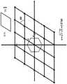
图2用图形描绘了时间、频率与Zak域之间的关系。Figure 2 graphically depicts the relationship between time, frequency and the Zak domain.

图3示出了六边形点阵的示例。中心区域处的六边形围住零点阵点周围的泰森多边形(Voronoi)区域。标注箭头的两个点阵点是最大矩形亚点阵的基础。Figure 3 shows an example of a hexagonal lattice. The hexagon at the central area encloses the Voronoi area around the zero lattice point. The two lattice points marked with arrows are the basis of the largest rectangular sub-lattice.

图4用图形描绘了Zak域中的信息网格的周期性和准周期性性质。Figure 4 graphically depicts the periodic and quasi-periodic properties of the information grid in the Zak domain.

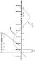
图5是OTFS波形的图形表示。Figure 5 is a graphical representation of the OTFS waveform.

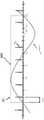
图6是经滤波的OTFS波形的图形表示。Figure 6 is a graphical representation of a filtered OTFS waveform.

图7是使用OTFS和OTFS-MC(多载波)的单个QAM符号的传输波形的图形比较。Figure 7 is a graphical comparison of the transmission waveforms of a single QAM symbol using OTFS and OTFS-MC (multi-carrier).

图8用图形描绘了其中Zak域和时间/频率Zak变换实现了位于时间实现与频率实现之间的信号空间实现的示例。Figure 8 graphically depicts an example where the Zak domain and the time/frequency Zak transform realize a signal space realization that lies between the time realization and the frequency realization.

图9示出了Zak至一般化Zak交织(interwining)变换的描绘。Figure 9 shows a depiction of the Zak to Generalized Zak interwining transformation.

图10示出了嵌套式点阵系统的示例，其中N＝3并且M＝2。Figure 10 shows an example of a nested lattice system where N=3 and M=2.

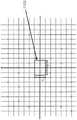
图11是对应于N＝3、M＝2、a＝1的线性调频(chirp)点阵的示例的图形描绘。虚线正方形指示零周围的清洁区域。11 is a graphical depiction of an example of a chirp lattice corresponding to N=3, M=2, a=1. The dashed square indicates the clean area around the zero.

图12是对应于斜率a＝1的连续Zak线性调频的模糊度函数的示例的描绘。12 is a depiction of an example of an ambiguity function corresponding to a continuous Zak chirp with slope a=1.

图13是无线通信方法的示例的流程图。13 is a flowchart of an example of a wireless communication method.

图14是无线通信方法的另一个示例的流程图。14 is a flowchart of another example of a wireless communication method.

图15是无线收发器装置的示例。15 is an example of a wireless transceiver device.

具体实施方式Detailed ways

为了使本公开的目的、技术解决方案和优点更明显，下文参考附图详细地描述各种实施例。除非另外指明，否则本文件的实施例和实施例中的特征可以彼此组合。In order to make the objects, technical solutions, and advantages of the present disclosure more apparent, various embodiments are hereinafter described in detail with reference to the accompanying drawings. Unless otherwise indicated, the embodiments of this document and features in the embodiments may be combined with each other.

章节标题在本文中用于提高描述的可读性并且绝不将技术的讨论或实施例仅限于相应的章节。Section headings are used herein to improve readability of the description and in no way limit the discussion or examples of techniques to the corresponding section.

诸如正交频分复用(OFDM)方案的传统多载波(MC)传输方案由两个参数表征：符号周期(或重复率)和子载波间隔。符号包括循环前缀(CP)，其大小典型地取决于使用OFDM调制方案的无线信道的延迟。换句话说，CP大小通常是基于信道延迟而固定的，并且如果符号收缩以增加系统率，则它简单地导致CP变成越来越大的开销。此外，紧密地放置的子载波可以导致载波间干涉，并且因此OFDM符号对子载波在不引起不可接受的干涉水平的情况下可以彼此放置多近具有实际限制，从而使得接收器更难成功地接收所发射的数据。Conventional multi-carrier (MC) transmission schemes such as Orthogonal Frequency Division Multiplexing (OFDM) schemes are characterized by two parameters: symbol period (or repetition rate) and subcarrier spacing. The symbols include a Cyclic Prefix (CP), the size of which typically depends on the delay of the wireless channel using the OFDM modulation scheme. In other words, the CP size is usually fixed based on the channel delay, and if the symbols are shrunk to increase the system rate, it simply causes the CP to become larger and larger overhead. Furthermore, closely placed sub-carriers can cause inter-carrier interference, and thus OFDM symbols have practical limits on how close sub-carriers can be placed to each other without causing unacceptable levels of interference, making it more difficult for a receiver to successfully receive transmitted data.

此外，在传统蜂窝通信网络中，发射设备在尝试使用随机访问机制的加入无线网络时使用正交码。这些正交码经过选择以使得能够在接收基站处清楚地检测到发射设备。Furthermore, in conventional cellular communication networks, transmitting devices use orthogonal codes when attempting to join a wireless network using a random access mechanism. These orthogonal codes are chosen to enable unambiguous detection of the transmitting device at the receiving base station.

所公开的技术的实施例部分地由以下实现启发：在无线设备与基站之间的信道因为无线设备的移动以及无线设备与基站之间的多路径回波而可能在延迟和多普勒域中受损时，无线装置可尝试加入网络。以类似的方式，雷达在检测可能移动的物体的操作的理论架构还可以得益于显示出与无线域中的随机访问波形类似的稳健性质的波形。本专利文件基于用于选择经滤波以产生模拟波形的数字域序列的技术以及滤波器响应与数字和模拟波形之间的数学关系(如其应用于其中实际系统尝试克服延迟和多普勒域失真的情形)，提供生成用于此类用途和其他用途的波形的理论基础。Embodiments of the disclosed technology are inspired in part by the realization that a channel between a wireless device and a base station may be in the delay and Doppler domains due to movement of the wireless device and multipath echoes between the wireless device and the base station. When compromised, the wireless device can attempt to join the network. In a similar manner, the theoretical architecture of radar's operation in detecting potentially moving objects may also benefit from waveforms that exhibit robust properties similar to random access waveforms in the wireless domain. This patent document is based on techniques for selecting digital-domain sequences filtered to produce analog waveforms and the mathematical relationship between filter responses and digital and analog waveforms (as applied to situations where practical systems attempt to overcome delay and Doppler-domain distortions). case), providing a rationale for generating waveforms for these and other uses.

本文件中公开的理论框架可以用来构建能够尤其克服上述问题的信号发射和接收设备。The theoretical framework disclosed in this document can be used to construct signal transmission and reception devices that can, inter alia, overcome the above-mentioned problems.

除其他技术外，本专利文件公开了一种点阵划分复用技术，在一些实施例中，该点阵划分复用技术可以用来实现能够执行多载波数字通信而不必依赖于CP的实施例。Among other techniques, this patent document discloses a lattice division multiplexing technique that, in some embodiments, can be used to implement embodiments capable of performing multi-carrier digital communications without necessarily relying on CP .

为便于说明，参考Zak变换来描述本文公开的许多实施例。然而，本领域技术人员将理解，实现方式也可以使用具有类似数学性质的其他变换。例如，此类变换可以包括能够表示为无穷级数的变换，其中每一项是平移了函数的整数的扩展与指数函数的乘积。For ease of illustration, many of the embodiments disclosed herein are described with reference to the Zak transform. However, those skilled in the art will understand that implementations may also use other transformations with similar mathematical properties. For example, such transformations may include transformations that can be represented as an infinite series, where each term is the product of an expansion of an integer shifted by the function and an exponential function.

图1示出了示例通信网络100，其中可以实现所公开的技术。网络 100可以包括基站发射器，所述基站发射器向一个或多个接收器102发射无线信号s(t)(例如，下行链路信号)，接收信号表示为r(t)，所述接收器可以位于多种位置，包括在建筑物内部或外部以及在移动的车辆中。接收器可以向基站发射上行链路发射，所述基站通常位于无线发射器附近。本文中描述的技术可以在接收器102处或在发射器(例如，基站) 处实现。FIG. 1 illustrates an example communication network 100 in which the disclosed techniques may be implemented. The network 100 may include base station transmitters that transmit wireless signals s(t) (eg, downlink signals), denoted r(t), to one or more receivers 102, the receivers Can be located in a variety of locations, including inside or outside buildings and in moving vehicles. A receiver may transmit uplink transmissions to a base station, which is typically located in the vicinity of the wireless transmitter. The techniques described herein may be implemented at receiver 102 or at a transmitter (eg, a base station).

无线网络中的信号传输可以通过描述时域、频域或延迟-多普勒域(例如，Zak域)中的波形来表示。由于这三者表示描述信号的三种不同方式，因此一个域中的信号可以经由变换而转换成另一个域中的信号。例如，时间-Zak变换可以用来从Zak域转换到时域。例如，频率-Zak变换可以用来从Zak域转换到频域。例如，傅里叶变换(或其逆变换)可以用来在时域与频域之间进行转换。Signal transmission in wireless networks can be represented by describing waveforms in the time domain, frequency domain, or delay-Doppler domain (eg, Zak domain). Since these three represent three different ways of describing a signal, a signal in one domain can be transformed into a signal in another domain via a transform. For example, the time-Zak transform can be used to convert from the Zak domain to the time domain. For example, the frequency-Zak transform can be used to convert from the Zak domain to the frequency domain. For example, the Fourier transform (or its inverse) can be used to convert between the time and frequency domains.

下面指定为“A”、“B”和“C”的章节提供在图2至图12中描绘的信号波形和曲线图的附加数学性质和实际使用。The sections designated "A", "B", and "C" below provide additional mathematical properties and practical uses of the signal waveforms and graphs depicted in Figures 2-12.

循环前缀(CP)的使用已经使得多载波波形(例如，OFDM)能够在频率选择信道中操作(当CP大于信道的延迟扩展时)，但在无线信道变得更加苛刻时，CP的长度需要增加，从而增加波形的开销。如在章节“A”和“B”中所述，所公开的技术的实施例可以用来执行多载波数字通信而不必依赖CP，以便有利地降低波形所需的开销。The use of a cyclic prefix (CP) has enabled multi-carrier waveforms (eg OFDM) to operate in frequency selective channels (when the CP is greater than the delay spread of the channel), but as wireless channels become more demanding, the length of the CP needs to increase , thereby increasing the waveform overhead. As described in Sections "A" and "B", embodiments of the disclosed technology can be used to perform multi-carrier digital communications without having to rely on CP, in order to advantageously reduce the overhead required for waveforms.

雷达波形的性能在受延迟扩展和多普勒扩展两者影响的信道(例如，被称为“双扩展信道”)中特别易受影响。如在章节“C”中所述，所公开的技术的实施例提供压缩的雷达波形，所述压缩雷达波形呈现均匀的时间功率轮廓和图钉状模糊度函数，其中在维度是自由参数的原点周围具有清洁穿孔区域，从而在延迟-多普勒表示中提供局部化。The performance of radar waveforms is particularly susceptible in channels that are affected by both delay spread and Doppler spread (eg, referred to as "double spread channels"). As described in Section "C", embodiments of the disclosed technology provide compressed radar waveforms that exhibit a uniform temporal power profile and a pushpin ambiguity function around an origin whose dimensions are free parameters Has clean perforated areas to provide localization in the delay-Doppler representation.

A0.从Zak理论的角度介绍OTFS调制A0. Introduction of OTFS modulation from the perspective of Zak theory

接下来的几个章节从Zak理论视角解释OTFS调制。这条阐述线将 OTFS的独立状态作为新颖调制技术推广到前沿并且暴露其独特的数学属性。这与将OTFS呈现为MC调制的预处理步骤的替代方法相比，稍微掩盖了OTFS的真实性质并且也牺牲了其一些独特优势。我们把注意力集中在以下核心理论主题：The next few chapters explain OTFS modulation from a Zak theory perspective. This elaboration line brings the independent state of OTFS to the forefront as a novel modulation technique and exposes its unique mathematical properties. This slightly masks the true nature of OTFS and also sacrifices some of its unique advantages compared to the alternative approach of presenting OTFS as a MC-modulated preprocessing step. We focus our attention on the following core theoretical themes:

(1)Heisenberg理论。(1) Heisenberg theory.

(2)Zak理论。(2) Zak theory.

(3)OTFS调制。(3) OTFS modulation.

(4)OTFS与多载波调制之间的辛傅里叶对偶关系，这是雷达理论与通信理论之间的一般关系的特殊情况。(4) The symplectic Fourier dual relationship between OTFS and multi-carrier modulation, which is a special case of the general relationship between radar theory and communication theory.

在进行详细阐述其演变之前，有益的是给出概述。在信号处理中，传统上呈现时域或频域中的信号(或波形)。每个表示暴露信号的不同属性。这两个实现之间的字典是傅里叶变换：Before elaborating on its evolution, it is helpful to give an overview. In signal processing, signals (or waveforms) are traditionally presented in the time or frequency domain. Each representation exposes a different property of the signal. The dictionary between these two implementations is the Fourier transform:

(0.1)

(0.1)

有趣的是，存在可以自然地实现信号的另一个域。这个域被称为延迟多普勒域。出于当前讨论的目的，这也被称为Zak域。以其最简单的形式，Zak信号是两个变量的函数

变量τ被称为延迟并且变量ν被称为多普勒。假设函数

随着具有周期ν_r的ν而呈周期性，并且随着具有周期τ_r的τ呈准周期性。准周期性条件由以下给出：Interestingly, there is another domain where signals can be implemented naturally. This domain is called the delayed Doppler domain. For the purposes of the current discussion, this is also known as the Zak domain. In its simplest form, the Zak signal is a function of two variables

The variable τ is called delay and the variable ν is called Doppler. Hypothetical function

Periodic with ν with period ν_r and quasi-periodic with τ with period τ_r . The quasiperiodic condition is given by:

(0.2)

(0.2)

其中，每个

假设周期满足尼奎斯特条件τ_r·ν_r＝1。Zak域信号通过被称为时间和频率Zak变换的正规变换

和

而与时域和频域信号相关。更准确地说，用

表示Zak信号的希尔伯特空间，时间和频率Zak变换是线性变换：Among them, each

It is assumed that the period satisfies the Nyquist condition τ_r ·ν_r =1. The Zak-domain signal undergoes a normal transformation known as the time and frequency Zak transform

and

It is related to time domain and frequency domain signals. More precisely, with

Representing the Hilbert space of a Zak signal, the time and frequency Zak transforms are linear:

(0.3)

(0.3)

(0.4)

(0.4)

成对的

和

建立傅里叶变换的因式分解

这个因式分解有时被称为Zak因式分解。Zak因式分解体现快速傅里叶变换算法的组合学。Zak变换的精确公式将在后面给出。而此刻，说成它们主要是几何投影就够了：时间Zak变换是沿多普勒变量的积分，并且相反地，频率Zak变换是沿延迟变量的积分。图2中描绘了不同的信号域以及在它们之间连接的变换。Pairs

and

Building the Factorization of the Fourier Transform

This factorization is sometimes called Zak factorization. Zak factorization embodies the combinatorics of fast Fourier transform algorithms. The exact formula of the Zak transform will be given later. At the moment, it is enough to say that they are mainly geometric projections: the time Zak transform is the integration along the Doppler variable, and conversely, the frequency Zak transform is the integration along the delay variable. The different signal domains and the transforms connected between them are depicted in FIG. 2 .

我们接下来给出OTFS调制的概述。关键要注意的是，Zak变换对 OTFS起到的作用与傅里叶变换对OFDM的作用相同。更具体地，在OTFS 中，信息位在延迟多普勒域上编码为Zak信号x(τ，ν)并且通过以下规则进行传输：We next give an overview of OTFS modulation. The key thing to note is that the Zak transform does the same thing for OTFS as the Fourier transform does for OFDM. More specifically, in OTFS, information bits are encoded as a Zak signal x(τ, ν) on the delayed Doppler domain and transmitted by the following rules:

(0.5)

(0.5)

其中w*_σx(τ，ν)表示使用被称为扭曲卷积(将在本文件中解释)的操作*_σ的、利用2D脉冲w(τ，ν)的二维滤波操作。使用Zak变换来完成到物理时域的转换。在频分多址FDMA和时分多址TDMA的情况下，公式 (0.5)应与类似公式进行对比。在FDMA中，信息位在频域上编码为信号x(f)并且通过以下规则进行传输：where w*_σx (τ,ν) represents a two-dimensional filtering operation with 2D pulses w(τ,ν) using an operation called warped convolution (explained in this document) *_σ . The conversion to the physical time domain is done using the Zak transform. In the case of frequency division multiple access FDMA and time division multiple access TDMA, equation (0.5) should be compared with similar equations. In FDMA, information bits are encoded in the frequency domain as a signal x(f) and transmitted by the following rules:

(0.6)FDMA(x)＝FT(w(f)*x(f))，(0.6) FDMA(x)=FT(w(f)*x(f)),

其中在频域上通过利用1D脉冲w(f)的线性卷积完成滤波(在标准OFDM w(f)等于sinc函数的情况下)。调制映射是傅里叶变换。在 TDMA中，信息位在时域上编码为信号x(t)并且通过以下规则进行传输：where filtering is done in the frequency domain by linear convolution with 1D pulses w(f) (in the case of standard OFDM w(f) equal to the sinc function). The modulation map is the Fourier transform. In TDMA, information bits are encoded in the time domain as a signal x(t) and transmitted by the following rules:

(0.7)TDMA(x)＝Id(w(t)*x(t))，(0.7) TDMA(x)=Id(w(t)*x(t)),

其中在时域上通过利用1D脉冲w(t)的线性卷积完成滤波。在这种情况下，调制映射是恒等式。where filtering is done in the time domain by linear convolution with 1D pulses w(t). In this case, the modulation map is the identity.

A1.Heisenberg理论A1. Heisenberg Theory

在这个章节中，我们介绍Heisenberg群和相关联的Heisenberg表示。这些构成信号处理的基本结构。概括地说，信号处理可以被计算成根据延迟和相位调制的Heisenberg操作来研究信号的各种实现。In this section, we introduce the Heisenberg group and the associated Heisenberg representation. These form the basic structure of signal processing. In a nutshell, signal processing can be computed to study various realizations of a signal in terms of the Heisenberg operation of delay and phase modulation.

A1.1 延迟多普勒平面A1.1 Delayed Doppler plane

最基本的结构是配备有以下标准辛形式的延迟多普勒平面

The most basic structure is a delayed Doppler plane equipped with the following standard symplectic form

(1.1)ω(υ₁，υ₂)＝v₁τ₂-τ₁v₂，(1.1)ω(υ₁ ,υ₂ )=v₁ τ₂ -τ₁ v₂ ,

其中，每个υ₁＝(τ₁，v₁)和υ₂(τ₂，v₂)。表达ω的另一种方式是将向量υ₁和υ₂布置成2×2矩阵的列，使得ω(υ₁，υ₂)等于矩阵行列式的加法逆元。where each υ₁ =(τ₁ , v₁ ) and υ₂ (τ₂ , v₂ ). Another way of expressing ω is to arrange the vectors υ₁ and υ₂ as columns of a 2×2 matrix such that ω(υ₁ ,υ₂ ) is equal to the additive inverse of the matrix determinant.

辛形式是反对称ω(υ₁，υ₂)＝-ω(υ₂，υ₁)，因此，具体地说，对于每个υ∈V，ω(υ，υ)＝0。我们也考虑以下计划形式：The symplectic form is antisymmetric ω(υ₁ , υ₂ ) = -ω(υ₂ , υ₁ ), so, in particular, for each υ∈V, ω(υ,υ)=0. We also consider the following program formats:

(1.2)β(υ₁，υ₂)＝v₁τ₂，(1.2)β(υ₁ ,υ₂ )=v₁ τ₂ ,

其中，每个υ₁＝(τ₁，ν₁)和υ₂＝(τ₂ν₂)。我们得到：where each υ₁ =(τ₁ , ν₁ ) and υ₂ =(τ₂ ν₂ ). we got:

(1.3)β(υ₁，υ₂)-β(υ₂，υ₁)＝ω(υ₁，υ₂)(1.3)β(υ₁ ,υ₂ )−β(υ₂ ,υ₁ )=ω(υ₁ ,υ₂ )

形式β应被认为是辛形式的“一半”。最终，用ψ(z)＝exp(2πiz)来表示标准一维傅里叶指数。Form beta should be considered "half" of the symplectic form. Finally, the standard one-dimensional Fourier index is expressed by ψ(z)=exp(2πiz).

A1.2 Heisenberg群A1.2 Heisenberg group

极化形式β产生被称为Heisenberg群的两步幂单群。作为一组， Heisenberg群被实现为Heis＝V×S¹，其中乘法规则由以下给出：The polarized form β produces a two-step power simple group known as the Heisenberg group. As a group, the Heisenberg group is realized as Heis=V×S¹ , where the multiplication rule is given by:

(1.4)(υ₁，z₁)·(υ₂，z₂)＝(υ₁+υ₂，exp(j2πβ(υ₁，υ₂))z₁z₂)，(1.4)(υ₁ , z₁ )·(υ₂ , z₂ )=(υ₁ +υ₂ , exp(j2πβ(υ₁ ,υ₂ ))z₁ z₂ ),

可以验证事实上规则(1.4)产生群结构：它是关联的，元素(0，1) 充当单位并且元素(υ，z)的逆元由以下给出：It can be verified that in fact rule (1.4) produces a group structure: it is associative, the element (0, 1) acts as the unit and the inverse of the element (υ, z) is given by:

(υ，z)^-1＝(-υ，exp(j2πβ(υ，υ))z^-1)(υ, z)⁻¹ =(−υ, exp(j2πβ(υ,υ))z⁻¹ )

最重要的是，Heisenberg群不可交换。一般来说， (υ₁，z₁)(υ₂，z₂)≠(υ₂，z₂)·(υ₁，z₁)。中心由形式(0，z)，z∈S¹的所有元素构成。乘法规则产生函数之间的群卷积运算：Most importantly, Heisenberg groups are not commutative. In general, (υ₁ , z₁ )(υ₂ , z₂ )≠(υ₂ , z₂ )·(υ₁ , z₁ ). The center consists of all elements of the form (0, z), z ∈ S¹ . The multiplication rule produces a group convolution operation between functions:

(1.5)

(1.5)

其中，每一对函数

我们将(1.5)称为Heisenberg卷积或扭曲卷积。我们注意到，扭曲卷积通过附加的相位因数exp(j2πβ(υ₁，υ₂)) 而不同于线性卷积。Among them, each pair of functions

We refer to (1.5) as Heisenberg convolution or warped convolution. We note that warped convolution differs from linear convolution by an additional phase factor exp(j2πβ(υ₁ ,υ₂ )).

A1.3 Heisenberg表示A1.3 Heisenberg said

Heisenberg群的表示理论相对简单。概括地说，通过固定中心的动作，存在唯一的(直至同构)不可约表示。这个唯一性被称为斯通-冯诺依曼 (Stone-von Neumann)性质。精确陈述在以下定理中概述：定理1.1 (Stone-von-Neumann定理)。存在唯一的(直至同构)不可约酉表示

使得

The representation theory of Heisenberg groups is relatively simple. In a nutshell, there exists a unique (up to isomorphic) irreducible representation by the action of a fixed center. This uniqueness is called the Stone-von Neumann property. The exact statement is outlined in the following theorem: Theorem 1.1 (Stone-von-Neumann theorem). There exists a unique (up to isomorphic) irreducible unitary representation

make

具体地说，Heisenberg表示是酉算子

的集合，对于每个υ∈V，满足可乘关系：Specifically, the Heisenberg representation is a unitary operator

The set of , for each υ∈V, satisfies the multiplicative relation:

(1.6)

(1.6)

其中，每个υ₁，υ₂∈V。换句话说，族中的各个算子之间的关系在 Heisenberg群的结构中编码。查看Heisenberg群的等效方式是作为线性变换

从而采用函数

并且将其发送到由以下给出的算子

where, for each υ₁ , υ₂ ∈V. In other words, the relationships between the various operators in the family are encoded in the structure of the Heisenberg group. The equivalent way to look at the Heisenberg group is as a linear transformation

thus using the function

and send it to the operator given by

(1.7)

(1.7)

可乘关系(1.6)转化成以下事实：II在函数的Heisenberg卷积与线性变换的组成之间交换，即，The multiplicative relation (1.6) translates into the fact that II is exchanged between the composition of the Heisenberg convolution of the function and the linear transformation, i.e.,

(1.8)

(1.8)

其中，每个

有趣的是，尽管是唯一的，但表示π容纳大量的实现。特别公知的是时间和频率实现，它们都是在实线

的复值函数的希尔伯特空间上定义的。对于每个

我们定义两个基本酉变换：Among them, each

Interestingly, despite being unique, the representation π accommodates a large number of realizations. Particularly well known are the time and frequency implementations, which are both in the solid line

is defined on the Hilbert space of complex-valued functions. for each

We define two basic unitary transformations:

(1.9)

(1.9)

(1.10)

(1.10)

其中，每个

变换L_x被称为延迟了x并且变换M_x被称为调制了 x。对于点ν＝(τ，ν)∈V，我们通过以下来定义Heisenberg表示的时间实现：Among them, each

Transform L_x is said to delay x and transform M_x is said to modulate x. For the point ν = (τ, ν) ∈ V, we define the time realization of the Heisenberg representation by:

(1.11)

(1.11)

其中我们使用符号

来指定算子在向量上的应用。在这个背景下，常用的是通过t(时间)来表示基本坐标函数。根据这个约定，(1.11)的右手侧采用显式形式exp

相互地，我们通过以下来定义 Heisenberg表示的频率实现：where we use the notation

to specify the application of the operator to the vector. In this context, it is commonly used to represent the basic coordinate function by t (time). By this convention, the right-hand side of (1.11) takes the explicit form exp

Reciprocally, we define the frequency realization of the Heisenberg representation by:

(1.12)

(1.12)

在这个背景下，习惯通过f(频率)来表示基本坐标函数。根据这个约定，(1.12)的右手侧采用显式形式exp

通过定理1.1，在具有在时间与频率Heisenberg动作之间转化的交织变换的意义上，时间和频率实现是同构的。在这种情况下，交织变换是傅里叶变换。In this context, it is customary to express the basic coordinate function by f (frequency). By this convention, the right-hand side of (1.12) takes the explicit form exp

By Theorem 1.1, time and frequency realizations are isomorphic in the sense of having an interleaving transformation that translates between time and frequency Heisenberg actions. In this case, the interleaving transform is the Fourier transform.

(1.13)

(1.13)

其中，每个

在以下意义上，时间和频率Heisenberg算子π_t(υ，z) 和π_f(υ，z)经由傅里叶变换进行交换：Among them, each

The time and frequency Heisenberg operators π_t (υ, z) and π_f (υ, z) are exchanged via the Fourier transform in the following sense:

(1.14)

(1.14)

其中，每个υ∈V。我们强调，从表示理论的角度来看，傅里叶变换的特有性质是交换等式(1.14)。where each υ∈V. We emphasize that, from the point of view of representation theory, the peculiar property of the Fourier transform is the exchange equation (1.14).

A2.Zak理论A2. Zak Theory

在这一章节，我们描述信号空间的Zak实现。Zak实现取决于参数的选择。这个参数是延迟多普勒平面中的临界采样的点阵。因此，首先我们花一些时间来熟悉一下点阵的基本理论。为简单起见，我们将注意力集中在矩形点阵上。In this section, we describe the Zak implementation of the signal space. Zak implementation depends on the choice of parameters. This parameter is a lattice of critical samples in the delayed Doppler plane. So, first let's take some time to get familiar with the basic theory of lattices. For simplicity, we focus on rectangular lattices.

A2.1延迟多普勒点阵A2.1 Delayed Doppler lattice

延迟多普勒点阵是一对线性无关向量g₁，g₂∈V的积分跨距。更详细地说，给定这样的一对，相关联的点阵是以下集合：A delayed Doppler lattice is the integral span of a pair of linearly independent vectors g₁ , g₂ ∈V. In more detail, given such a pair, the associated lattice is the following set:

(2.1)

(2.1)

向量ɡ₁和ɡ₂被称为点阵基本向量。方便的是将基本向量布置成矩阵 G的第一列和第二列，即：The vectors ɡ₁ and ɡ₂ are called lattice basis vectors. It is convenient to arrange the basis vectors into the first and second columns of the matrix G, i.e.:

(2.2)

(2.2)

被称为基本矩阵。通过这种方式，点阵

也就是，根据矩阵 G的标准点阵的图像。按照定义，点阵的体积就是基本域的面积，其等于G的行列式的绝对值。每个点阵容纳辛倒点阵，亦称正交互补点阵，我们表示为Λ^⊥。Λ^⊥的定义是：is called the fundamental matrix. In this way, the lattice

That is, according to the image of the standard lattice of matrix G. By definition, the volume of a lattice is the area of the fundamental domain, which is equal to the absolute value of the determinant of G. Each point array is a Nassin inverted lattice, also known as an orthogonal complementary lattice, which we denote as Λ^⊥ . The definition of Λ^⊥ is:

(2.3)

(2.3)

如果

则说Λ是欠采样的；如果Λ＝Λ^⊥，则说Λ是临界采样的。替代地，欠采样的点阵使得其基本域的体积≥1。从现在开始，我们仅考虑欠采样的点阵。给定点阵Λ，我们将其最大矩形亚点阵定义为

其中：if

Then Λ is said to be undersampled; if Λ=Λ^⊥ , then Λ is said to be critically sampled. Alternatively, the lattice is undersampled such that the volume of its base domain is≥ 1. From now on, we will only consider undersampled lattices. Given a lattice Λ, we define its largest rectangular sublattice as

in:

(2.4)τ_r＝arg min{τ＞0：(τ，0)∈Λ}，(2.4)τ_r =arg min{τ>0: (τ, 0)∈Λ},

(2.5)ν_r＝arg min{v＞0：(0，v)∈Λ}，(2.5) ν_r = arg min {v>0: (0, v)∈Λ},

当τ_r或v_r是无限的时，我们定义Λ_r＝{0}。如果Λ＝Λ_r，则说点阵Λ是矩形的。显然，矩形点阵的亚点阵也是矩形的。如果τ_rν_r≥1，则矩形点阵是欠采样的。临界采样的点阵的标准示例为

其由单位矩阵生成：When τ_r or v_r is infinite, we define Λ_r = {0}. If Λ=_Λr , the lattice Λ is said to be rectangular. Obviously, the sublattice of a rectangular lattice is also rectangular. A rectangular lattice is undersampled if τ_r ν_r≥ 1. A standard example of a critically sampled lattice is

It is generated by the identity matrix:

(2.6)

(2.6)

不是矩形的临界采样的点阵的重要示例是六边形点阵Λ_hex，见图3，其由基本矩阵生成：An important example of a critically sampled lattice that is not rectangular is the hexagonal lattice_Λhex , see Figure 3, which is generated by the fundamental matrix:

(2.7)

(2.7)

其中

六边形点阵的有趣属性在于，在所有临界采样的点阵中，它具有邻近点之间的最长距离。Λ_hex的最大矩形亚点阵由g₁和 2g₂-g₁生成，见图3中用箭头标注的两个点阵点。从现在开始，我们仅考虑矩形点阵。in

An interesting property of the hexagonal lattice is that it has the longest distance between adjacent points of all critically sampled lattices. The largest rectangular sublattice of_Λhex is generated by g₁ and 2g₂ -g₁ , see the two lattice points marked with arrows in Fig. 3. From now on, we will only consider rectangular lattices.

A2.2Zak波形A2.2Zak waveform

Zak实现通过选择临界采样的点阵来参数化：The Zak implementation is parameterized by choosing a critically sampled lattice:

(2.8)

(2.8)

其中τ_r·ν_r＝1。Zak实现中的信号被称为Zak信号。通过固定点阵Λ， Zak信号是满足以下准周期性条件的函数

where τ_r ·ν_r =1. Signals in Zak implementations are called Zak signals. By fixing the lattice Λ, the Zak signal is a function that satisfies the following quasi-periodic conditions

(2.9)

(2.9)

其中，每个υ∈V和λ∈Λ。通过写出λ＝(kτ_r，lν_r)，条件(2.9) 采取具体形式：where each υ∈V and λ∈Λ. By writing λ = (kτ_r , lν_r ), condition (2.9) takes the concrete form:

(2.10)

(2.10)

也就是说，

是沿多普勒维度的具有周期v_r的周期函数，并且是沿着延迟维度的具有准周期τ_r的准周期函数。总而言之，我们用

来表示 Zak信号的希尔伯特空间。That is,

is a periodic function with period v_r along the Doppler dimension, and is a quasi-periodic function with a quasi-period τ_r along the delay dimension. All in all, we use

to represent the Hilbert space of the Zak signal.

A2.3 Heisenberg动作A2.3 Heisenberg action

Zak信号的希尔伯特空间支持Heisenberg表示的实现。给定元素 u∈V，对应的Heisenberg算子π_z(u)由以下给出：The Hilbert space of the Zak signal supports the implementation of the Heisenberg representation. Given an element u ∈ V, the corresponding Heisenberg operator π_z (u) is given by:

(2.11)

(2.11)

其中，每个

换句话说，元素u通过二维移位以及线性相位的调制来起作用。在元素u属于点阵的情况下，Heisenberg动作简化。直接计算表明，在这种情况下，u＝λ∈Λ的动作采取以下形式：Among them, each

In other words, the element u functions by a two-dimensional shift and modulation of the linear phase. In the case where the element u belongs to a lattice, the Heisenberg action simplifies. Direct computation shows that, in this case, the action for u = λ∈Λ takes the form:

(2.12)

(2.12)

换句话说，算子π_z(λ)跟与点λ相关联的辛傅里叶指数相乘。因此，脉冲函数

的扩展动作由以下给出：In other words, the operator π_z (λ) is multiplied by the symplectic Fourier exponent associated with the point λ. Therefore, the impulse function

The extension action for is given by:

(2.13)

(2.13)

其中，每个

事实上，

也就是说，扩展动作由脉冲h与波形

的扭曲函数给出。Among them, each

In fact,

That is, the expansion action consists of the pulse h and the waveform

The twist function of .

A2.4 Zak变换A2.4 Zak Transform

在Zak信号与时间/频率信号之间存在典型的交织变换，在本文件中被称为时间/频率Zak变换。我们用以下来表示它们：There is a typical interleaving transform between a Zak signal and a time/frequency signal, referred to in this document as a time/frequency Zak transform. We denote them by:

(2.14)

(2.14)

(2.15)

(2.15)

事实证明，时间/频率Zak变换是沿着相反维度(reciprocal dimension) 的基本几何投影，见图4。变换的公式如下：It turns out that the time/frequency Zak transform is a fundamental geometric projection along the reciprocal dimension, see Figure 4. The formula for the transformation is as follows:

(2.16)

(2.16)

(2.17)

(2.17)

其中，每个

换句话说，对于每个时间点，时间Zak变换是沿着多普勒维度(取DC分量)的积分。相反地，频率Zak变换是沿着延迟维度的傅里叶变换。逆变换的公式如下：Among them, each

In other words, for each time point, the temporal Zak transform is the integration along the Doppler dimension (taking the DC component). Conversely, the frequency Zak transform is a Fourier transform along the delay dimension. The formula for the inverse transform is as follows:

(2.18)

(2.18)

(2.19)

(2.19)

其中，每个

从现在开始，我们将仅集中在时间Zak变换并且用

来表示它。作为交织变换，

在两个Heisenberg算子π_z(υ，z) 和π_t(υ，z)之间交换，即：Among them, each

From now on, we will focus only on the temporal Zak transform and use

to represent it. As an interleaving transform,

Swap between the two Heisenberg operators π_z (υ, z) and π_t (υ, z), namely:

(2.20)

(2.20)

其中，每个υ∈V。从表示理论的角度来看，Zak变换的特有性质是交换等式(2.20)。where each υ∈V. From the standpoint of representation theory, the characteristic property of the Zak transform is the exchange equation (2.20).

A2.5 标准Zak信号A2.5 Standard Zak Signal

我们的目标是描述窗口函数的Zak表示。Our goal is to describe the Zak representation of the window function.

(2.21)

(2.21)

这个函数通常被用作多载波调制(没有CP)中的发生器波形。公式 (2.18)的直接应用表明

由以下给出：This function is often used as a generator waveform in multicarrier modulation (without CP). A direct application of formula (2.18) shows that

is given by:

(2.22)

(2.22)

可以表明，对于每个a，b∈[0，1)，P(aτ_r，bv_r)＝1，这意味着它具有恒定模数1，其中相位由沿着τ的常规阶梯函数给出，并且恒定阶梯由多普勒坐标v给出。注意P沿着延迟以每个整数点在相位上跳跃时的不连续。这个相位不连续是矩形窗口p在边界处的不连续的Zak域表现。It can be shown that for each a, b ∈ [0, 1), P(aτ_r , bv_r ) = 1, which means it has aconstant modulus 1, where the phase is given by the regular step function along τ, And the constant step is given by the Doppler coordinate v. Note the discontinuity as P jumps in phase at every integer point along the delay. This phase discontinuity is the Zak-domain representation of the discontinuity of the rectangular window p at the boundary.

A3.OTFSA3.OTFS

OTFS收发器结构取决于以下参数的选择：临界采样的点阵

滤波函数

以及由

指定的信息网格。我们假设滤波函数因式分解为w(τ，ν)＝w_τ(τ)w_ν(ν)，其中延迟和多普勒因数分别是相对于Δτ＝τ_r/N和Δν＝ν_r/M的平方根尼奎斯特。我们将信息位编码为具有周期(N，M)的QAM符号x＝x[nΔτ，mΔν]的周期性2D序列。将x乘以标准Zak信号P，我们得到Zak信号xP。考虑xP的具体方式是作为有限序列x[nΔτ，mΔν]的唯一准周期性扩展，其中n＝0、……、N–1并且 m＝0、……、M–1。我们将经调制的传输波形定义为：The OTFS transceiver structure depends on the choice of the following parameters: Lattice for critical sampling

filter function

and by

The specified information grid. We assume that the filter function is factored as w(τ, ν) = w_τ (τ)w_ν (ν), where the delay and Doppler factors are relative to Δτ = τ_r /N and Δν = ν_r /M, respectively The square root of Nyquist. We encode the information bits as a periodic 2D sequence of QAM symbols x=x[nΔτ, mΔν] with period (N, M). Multiplying x by the standard Zak signal P, we get the Zak signal xP. A specific way to consider xP is as the only quasi-periodic extension of the finite sequence x[nΔτ, mΔν], where n=0, . . . , N−1 and m=0, . . . , M−1. We define the modulated transmission waveform as:

(3.1)

(3.1)

概括地说，调制规则分三步进行。在第一步骤中，将信息块x准周期化，因此将其变换成离散Zak信号。在第二步骤中，通过由利用脉冲w 的扭曲卷积限定的2D滤波过程来使信号的带宽和持续时间成形。在第三步骤中，通过应用Zak变换来将经滤波的信号转换到时域。为了更好地理解传输波形的结构，我们将几个简单的代数操作应用于(3.1)。首先，我们注意到，作为交织子(公式(2.20))，Zak变换遵循以下关系：In a nutshell, the modulation rule works in three steps. In a first step, the information block x is quasi-periodic and thus transformed into a discrete Zak signal. In a second step, the bandwidth and duration of the signal are shaped by a 2D filtering process defined by twisted convolution with pulse w. In a third step, the filtered signal is converted to the time domain by applying the Zak transform. To better understand the structure of the transmission waveform, we apply a few simple algebraic operations to (3.1). First, we notice that, as an interleaver (Equation (2.20)), the Zak transform follows the relationship:

(3.2)

(3.2)

第二，我们注意到，因式分解w(τ，v)＝w_τ(τ)w_v(v)可以表达为扭曲卷积w＝w_τ*_σw_v。因此，可以写出：Second, we note that the factorization w(τ, v) = w_τ (τ) w_v (v) can be expressed as a warped convolution w = w_τ *_σ w_v . Therefore, one can write:

(3.3)

(3.3)

其中W_t＝FT^-1(w_v)并且*代表时间上的线性卷积。我们将波形

称为裸OTFS波形。我们从公式(3.3)中看出，通过在时间上开窗口然后利用脉冲进行卷积而从裸波形中获得传输波形。这个级联的操作是Zak域中的2D滤波的时间表示。在x被支持在单个网格点上(即，由单个QAM符号构成)的情况下，即，x＝δ(nΔτ，mΔν)，研究裸OTFS 波形的结构是有益的。在这种情况下，可以表明裸波形采取以下形式：where W_t =FT^-1 (w_v ) and * represents a linear convolution in time. We will waveform

Called a bare OTFS waveform. We see from equation (3.3) that the transmitted waveform is obtained from the bare waveform by windowing in time and then convolving with the pulse. This cascaded operation is the temporal representation of 2D filtering in the Zak domain. In the case where x is supported on a single grid point (ie, consists of a single QAM symbol), ie, x = δ(nΔτ, mΔν), it is beneficial to study the structure of the bare OTFS waveform. In this case, it can be shown that the naked waveform takes the form:

(3.4)

(3.4)

换句话说，裸波形是脉冲率

的经移位和相位调制的无限Δ脉冲串，其中移位由延迟参数n决定并且调制由多普勒参数m决定。与单个QAM符号对应的裸以及经滤波的OTFS波形分别在图5和图6中描绘。接下来，我们描述解调制映射。给定接收到的波形

通过以下规则来定义其解调制图像

In other words, the naked waveform is the pulse rate

A shifted and phase modulated infinite delta burst of , where the shift is determined by the delay parameter n and the modulation is determined by the Doppler parameter m. The raw and filtered OTFS waveforms corresponding to a single QAM symbol are depicted in Figures 5 and 6, respectively. Next, we describe the demodulation mapping. Given the received waveform

Its demodulated image is defined by the following rules

(3.5)

(3.5)

其中w^★是由

给出的匹配的滤波器。我们通常结合附加采样步骤y处于(nΔτ，mΔν)，其中n＝0，...，N-1，并且m＝0，...，M-1。where w^★ is given by

given matched filter. We typically combine additional sampling steps y at (nΔτ, mΔν), where n=0, . . . , N-1, and m=0, . . . , M-1.

A3.1 OTFS信道模型A3.1 OTFS channel model

OTFS信道模型是在存在信道H的情况下输入变量x与输出变量y 之间的显式关系。我们假设信道变换被定义为H＝Π_t(h)，其中h＝h(τ，ν)是延迟多普勒脉冲响应。这意味着，给定传输波形

接收到的波形

由以下给出：The OTFS channel model is an explicit relationship between the input variable x and the output variable y in the presence of the channel H. We assume that the channel transformation is defined as H = Π_t (h), where h = h(τ, ν) is the delayed Doppler impulse response. This means that, given the transmission waveform

received waveform

is given by:

(3.6)

(3.6)

如果我们将传输波形表示为

那么直接计算表明：If we represent the transmission waveform as

Then the direct calculation shows that:

(3.7)

(3.7)

如果我们表示h_w＝w^★*_σh*_σw，那么我们可以用以下形式写出输入 -输出关系：If we denote h_w = w^★ *_σ h*_σ w, then we can write the input-output relationship in the form:

(3.8)y＝h_w*_σx·P，(3.8)_y =hw*_σx ·P,

延迟多普勒脉冲h_w表示在QAM符号通过OTFS收发器循环进行调制和解调制时与这些符号交互的经滤波的信道。可以表明，在一些适当的假设下，h_w由h*w⁽²⁾很好地逼近，其中*代表线性卷积并且w⁽²⁾＝w^★*w 是线性自相关函数。在信道不重要的情况下，也就是说，h＝δ(0，0)，我们得到h_w＝w^★*_σw～w⁽²⁾，因此在采样之后我们得到(近似)完美的重建关系：The delayed Doppler pulse hw represents the filtered channel that interacts with the QAM symbols as they are cyclically modulated and demodulated by the_OTFS transceiver. It can be shown that, under some appropriate assumptions, hw is well approximated by h*_w⁽²⁾ , where * represents a linear convolution and w⁽²⁾ = w^★ *w is a linear autocorrelation function. In the case where the channel is not important, that is, h = δ(0, 0), we get h_w = w^* *_σ w ~ w⁽²⁾ , so after sampling we get an (approximately) perfect reconstruction relation :

(3.9)y[nΔτ，mΔv]～x[nΔτ，mΔv]，(3.9) y[nΔτ, mΔv]～x[nΔτ, mΔv],

其中，每个n＝0，...，N-1以及m＝0，..，M-1。where each n=0, . . , N-1 and m=0, . . , M-1.

A4.辛傅里叶对偶A4. Symmetric Fourier Dual

在这个章节中，我们描述可以借助于辛傅里叶对偶表达为临界采样的MC调制上的预处理步骤的OTFS调制的变体。我们将这个变体称为 OTFS-MC。为了具体起见，我们仅针对没有CP的OFDM的情况开发了显式公式。In this section, we describe a variant of OTFS modulation that can be expressed as a preprocessing step on critically sampled MC modulation by means of symplectic Fourier duality. We call this variant OTFS-MC. To be specific, we only develop explicit formulations for the case of OFDM without CP.

A4.1 辛傅里叶变换A4.1 Sympic Fourier Transform

我们用L₂(V)来表示向量空间V上的平方可积函数的希尔伯特空间。对于每个υ∈V，我们将由v参数化的辛指数(波函数)定义为由以下给出的函数

(4.1)ψ_υ(u)＝exp(j2πω(υ，u))We denote the Hilbert space of square-integrable functions on the vector space V by L₂ (V). For each υ∈V, we define the symplectic index (wave function) parameterized by v as the function given by

(4.1)ψ_υ (u)=exp(j2πω(υ, u))

其中，每个u∈V。具体地，如果υ＝(τ，ν)并且u＝(τ′，ν′)，那么ψ_υ(u)＝exp(j2π(ντ′-τν′))。使用辛指数，我们将辛傅里叶变换定义为由以下给出的酉变换SF：L₂(V)→L₂(V)：where each u ∈ V. Specifically, if υ=(τ,ν) and u=(τ′,ν′), then_ψυ (u)=exp(j2π(ντ′−τν′)). Using the symplectic index, we define the symplectic Fourier transform as the unitary transform SF given by: L₂ (V) → L₂ (V):

(4.2)

(4.2)

辛傅里叶变换满足各种感兴趣的性质(很多类似于标准欧几里得傅里叶变换)。辛傅里叶变换在线性卷积与函数的乘法之间转换，也就是说：The symplectic Fourier transform satisfies various properties of interest (many are similar to the standard Euclidean Fourier transform). The symplectic Fourier transform converts between linear convolution and multiplication of functions, that is:

(4.3)SF(g₁*g₂)＝SF(g₁)·SF(g₂)，(4.3) SF(g₁ *g₂ )=SF(g₁ )·SF(g₂ ),

对于每个g₁，g₂∈L₂(V)。给定点阵

辛傅里叶变换相对于辛倒点阵Λ^⊥将Λ上的采样函数映射到周期函数。也就是说，如果g被采样并且G＝SF(g)，那么对于每个υ∈V和λ^⊥∈Λ^⊥，G(υ+λ^⊥)＝G(υ)。在Λ被临界采样的情况下，这个关系采取更简单的形式，因为Λ^⊥＝Λ。最终，不同于其欧几里得对应方，辛傅里叶变换等于其逆变换，也就是SF＝SF^-1。For each g₁ , g₂ ∈ L₂ (V). given lattice

The symplectic Fourier transform maps a sampling function on Λ to a periodic function with respect to the symplectic inverse lattice Λ^⊥ . That is, if g is sampled and G=SF(g), then for each^υ∈V and^{λ⊥∈Λ⊥} , G(υ+^λ⊥ )=G(υ). In the case where Λ is critically sampled, this relation takes a simpler form, since Λ^⊥ = Λ. Ultimately, unlike its Euclidean counterpart, the symplectic Fourier transform is equal to its inverse, ie SF=SF^-1 .

A4.2 OTFS-MCA4.2 OTFS-MC

主要出发点是滤波脉冲w的定义及其应用于QAM符号的方式。为了定义MC滤波脉冲，我们考虑点阵

上的经采样的窗口函数

我们将w定义为W两倍的辛傅里叶：The main starting point is the definition of the filter pulse w and the way it applies to QAM symbols. To define the MC filter pulse, we consider the lattice

sampled window function on

We define w as the symplectic Fourier of twice W:

(4.4)w＝SF(W)，按照定义，w是V的周期函数，从而满足对于每个υ∈V以及λ∈Λ，ww(υ+λ)＝w(υ)。通常，W被视为具有跨越某一带宽B＝M·ν_r和持续时间T＝N·τ_r的0/1值的正方形窗口。在这种情况下，w将转为相对于网格

成尼奎斯特的狄利克雷辛格(Dirichlet sinc)函数，其中：(4.4) w = SF(W), w is by definition a periodic function of V such that for each υ∈V and λ∈Λ, ww(υ+λ)=w(υ). Typically, W is viewed as a square window with 0/1 values spanning some bandwidth B=M·ν_r and duration T=N·τ_r . In this case w will be turned relative to the grid

into Nyquist's Dirichlet sinc function, where:

(4.5)Δτ＝τ_r/N，(4.5) Δτ=τ_r /N,

(4.6)Δν＝ν_r/M，(4.6)Δν=ν_r /M,

更复杂的窗口设计可以包括沿着边界渐缩并且还包括伪随机加扰相位值。如前所述，将比特位编码为具有周期(N，M)的QAM符号 x＝x[nΔτ，mΔν]的2D周期性序列。通过以下规则来定义传输波形：More complex window designs may include tapering along the boundaries and also include pseudo-randomly scrambled phase values. As before, the bits are encoded as a 2D periodic sequence of QAM symbols x=x[nΔτ, mΔν] with period (N, M). The transmission waveform is defined by the following rules:

(4.7)

(4.7)

换句话说，OTFS-MC调制分三步进行。第一步骤，借助于利用周期性脉冲w的周期卷积对周期性序列进行滤波。第二步骤，通过与Zak信号P相乘来将经滤波的函数转换成Zak信号。第三步骤，借助于Zak变换将Zak信号转换到物理时域中。我们强调与公式(3.1)的差异，其中序列首先乘以P并且然后通过利用非周期性脉冲的扭曲卷积进行滤波。重点是，不同于(3.1)，通过与MC调制的辛傅里叶对偶来使公式(4.7) 相关。为明白这一点，我们首先注意到，w*x＝SF(W·X)，其中X＝SF(x)。这意味着我们可以写出：In other words, OTFS-MC modulation proceeds in three steps. In the first step, the periodic sequence is filtered by means of periodic convolution with periodic pulses w. In the second step, the filtered function is converted into a Zak signal by multiplying with the Zak signal P. In the third step, the Zak signal is converted into the physical time domain by means of the Zak transform. We emphasize the difference from equation (3.1), where the sequence is first multiplied by P and then filtered by twisted convolution with aperiodic pulses. The point is that, unlike (3.1), equation (4.7) is related by a symplectic Fourier dual with MC modulation. To understand this, we first note that w*x=SF(W·X), where X=SF(x). This means we can write:

(4.8)

(4.8)

按照定义，第一等式是辛傅里叶变换并且第二等式是按照公式 (2.12)。我们表示X_W＝W·X。通过建立这个关系，我们可以将(4.7) 发展为以下形式：By definition, the first equation is the symplectic Fourier transform and the second equation is according to equation (2.12). We denote X_W = W·X. By establishing this relationship, we can develop (4.7) into the following form:

(4.9)

(4.9)

其中第三等式是Zak变换的交织性质，并且按照定义，第四等式是

在没有CP的OFDM的情况下，脉冲p由沿着间隔[0，τ_r]的正方形窗口给出。因此，(4.9)中的最后表达可以显式地写成：where the third equation is the interleaving property of the Zak transform, and by definition the fourth equation is

In the case of OFDM without CP, the pulse p is given by a square window along the interval [0,_τr ]. Therefore, the final expression in (4.9) can be written explicitly as:

(4.10)

(4.10)

(4.10)的最后表达可以被认为是傅里叶系数X_W的(窗口)序列的 MC调制。有趣的是将对应于单个QAM符号的OTFS和OTFS-MC的传输波形进行比较。这两个结构在图7中描绘。主要结构差异是在OTFS-MC 的情况下，在网格点

处存在不连续性。The final expression of (4.10) can be thought of as the MC modulation of the (window) sequence of Fourier coefficients_XW . It is interesting to compare the transmission waveforms of OTFS and OTFS-MC corresponding to a single QAM symbol. These two structures are depicted in FIG. 7 . The main structural difference is that in the case of OTFS-MC, at grid points

There are discontinuities.

B0.从实现理论角度介绍OTFS收发器操作B0. Introduce OTFS transceiver operation from the perspective of implementation theory

在后续章节中，我们从实现理论的角度介绍OTFS收发器的又一数学解释。概括地说，在这种方法中，将波形的信号空间视作Heisenberg 群的表示空间或等效地视作配备有Heisenberg算子的集合的希尔伯特空间，每一者与延迟多普勒平面中的不同点相关联。这个表示空间容纳许多表示。两个标准的实现是时间和频率实现，并且它们通过一维傅里叶变换进行相关。在通信理论中，TDMA收发器结构天然地适合于时间实现，因为QAM符号沿着时间坐标复用，而OFD收发器结构天然地适合于频率实现，因为QAM符号沿着频率坐标复用。主要观察在于，存在位于时间与频率实现之间的规范实现，被称为Zak实现。有趣的是，Zak实现中的波形被表示为满足某些准周期性条件的二维延迟多普勒域上的函数。这个注意的主要信息在于，Zak实现天然地适合于OTFS收发器。从这个角度看OTFS收发器减少了它在其他现有的收发器结构之中的新颖和独立优势。为方便起见，我们在下表中概述了在这个注意中呈现的主要公式：In subsequent chapters, we introduce yet another mathematical interpretation of OTFS transceivers from the perspective of implementation theory. In general terms, in this approach, the signal space of a waveform is treated as a representation space of a Heisenberg group or equivalently as a Hilbert space equipped with a set of Heisenberg operators, each with delay Doppler Different points in the plane are associated. This presentation space holds many presentations. The two standard realizations are time and frequency realizations, and they are correlated by a one-dimensional Fourier transform. In communication theory, the TDMA transceiver structure is naturally suitable for time implementation because QAM symbols are multiplexed along the time coordinate, while the OFD transceiver structure is naturally suitable for frequency implementation because QAM symbols are multiplexed along the frequency coordinate. The main observation is that there are canonical implementations that lie between time and frequency implementations, known as Zak implementations. Interestingly, the waveforms in Zak's implementation are represented as functions on the two-dimensional delayed Doppler domain satisfying certain quasi-periodic conditions. The main message of this note is that Zak implementations are naturally suitable for OTFS transceivers. Looking at the OTFS transceiver from this perspective reduces its novel and independent advantages over other existing transceiver architectures. For convenience, we outline the main formulae presented in this note in the table below:

(0.1)

(0.1)

其中Q是准的缩写并且Z是Zak的缩写。where Q is an abbreviation for Quasi and Z is an abbreviation for Zak.

B1.数学预备知识B1. Preliminary knowledge of mathematics

B1.1 延迟多普勒平面B1.1 Delayed Doppler Plane

设

为配备有由以下给出的标准辛双线性形式

的延迟多普勒平面：Assume

is equipped with the standard symplectic bilinear form given by

The delayed Doppler plane of:

(1.1)ω（υ₁，υ₂）＝v₁τ₂-τ₁v₂，(1.1)ω(υ₁ ,υ₂ )=v₁ τ₂ -τ₁ v₂ ,

其中，每个υ₁＝(τ₁，ν₁)以及υ₂＝(τ₂，ν₂)。表达ω的另一种方式是将向量v₁和v₂布置成2×2矩阵的列。辛配对ω(v₁，v₂)等于这个矩阵的行列式的加法逆元，即：where each υ₁ =(τ₁ , ν₁ ) and υ₂ =(τ₂ , ν₂ ). Another way to express ω is to arrange the vectors v1 and v2 as columns of_a2x2 matrix. The symplectic pair ω(v₁ , v₂ ) is equal to the additive inverse of the determinant of this matrix, namely:

我们注意到，辛形式是反对称的，即，ω(υ₁，υ₂)＝-ω(υ₂，υ₁)，因此，具体地说，对于每个v∈V，ω(υ，υ)＝0。另外，我们考虑由以下给出的极化形式

We note that the symplectic form is antisymmetric, ie, ω(υ₁ ,υ₂ ) = -ω(υ₂ ,υ₁ ), so, specifically, for every v∈V, ω(υ,υ )=0. Additionally, we consider the polarization form given by

(1.2)β(υ₁，υ₂)＝v₁τ₂，(1.2)β(υ₁ ,υ₂ )=v₁ τ₂ ,

其中，每个υ₁＝(τ₁，ν₁)以及υ₂＝(τ₂，ν₂)。我们得到：where each υ₁ =(τ₁ , ν₁ ) and υ₂ =(τ₂ , ν₂ ). we got:

(1.3)β(υ₁，υ₂)-β(υ₂，υ₁)＝ω(υ₁，υ₂)，(1.3)β(υ₁ ,υ₂ )−β(υ₂ ,υ₁ )=ω(υ₁ ,υ₂ ),

形式β应被认为是辛形式的“一半”。最终，用ψ(z)＝exp(2πiz)来表示标准一维傅里叶指数。Form beta should be considered "half" of the symplectic form. Finally, the standard one-dimensional Fourier index is expressed by ψ(z)=exp(2πiz).

B1.2 延迟多普勒点阵B1.2 Delayed Doppler Lattice

参考以上章节A2.1。Refer to Section A2.1 above.

B1.3 Heisenberg群B1.3 Heisenberg group

极化形式

产生被称为Heisenberg群的两步幂单群。作为一组，Heisenberg群被实现为Heis＝V×S¹，其中乘法规则由以下给出：polarized form

Produces a two-step power simple group known as the Heisenberg group. As a group, the Heisenberg group is realized as Heis=V×S¹ , where the multiplication rule is given by:

(1.11)(υ₁，z₁)·(υ₂，z₂)＝(υ₁+υ₂，ψ(β(υ₁，υ₂))z₁z₂)，(1.11)(υ₁ , z₁ )·(υ₂ , z₂ )=(υ₁ +υ₂ ,ψ(β(υ₁ ,υ₂ ))z₁ z₂ ),

可以验证事实上规则(1.11)引起群结构，即，它是关联的，元素(0， 1)充当单位并且(υ，z)的逆元是(-υ，ψ(β(υ，υ))z^-1)。我们注意到，Heisenberg 群是不可交换的，即，

不一定等于

群的中心由形式(0，z)， z∈S¹的所有元素构成。乘法规则产生函数之间的群卷积运算：It can be verified that in fact the rule (1.11) gives rise to a group structure, i.e. it is associative, the element (0, 1) acts as the unit and the inverse of (υ, z) is (-υ, ψ(β(υ, υ)) z^-1 ). We note that the Heisenberg group is not commutative, i.e.,

not necessarily equal to

The center of the group consists of all elements of the form (0, z), z ∈ S¹ . The multiplication rule produces a group convolution operation between functions:

(1.12)

(1.12)

对于每一对函数

(Heis)。我们将卷积运算

称为Heisenberg 卷积或扭曲卷积。for each pair of functions

(Heis). We will convolution operation

It is called Heisenberg convolution or warped convolution.

Heisenberg群容纳许多有限子商群。每个这样的群与对(Λ，∈)的选择相关联，其中

是欠采样的点阵并且∈：Λ→S¹是满足以下条件的映射：Heisenberg groups hold many finite subquotient groups. Each such group is associated with the choice of the pair (Λ, ∈), where

is an undersampled lattice and ∈:Λ→S¹ is a mapping satisfying the following conditions:

(1.13)∈(λ₁+λ₂)＝∈(λ₁)∈(λ₂)ψ(β(λ₁，λ₂))，(1.13)∈(λ₁ +λ₂ )=∈(λ₁ )∈(λ₂ )ψ(β(λ₁ ,λ₂ )),

使用∈，我们定义由

给出的部分映射

可以验证(1.13)暗示

是群同态，也就是说，

总而言之，映射∈将Λ的部分同态嵌入定义为Heisenberg群的子群。我们将∈称为Heisenberg字符并且将对(Λ，∈)称为Heisenberg点阵。简单的示例是在点阵Λ为矩形时，即Λ＝Λ_r。在这种情形下，β|Λ＝0，因此我们可以采取∈＝1，对应于不重要的嵌入

更复杂的示例是配备有∈_hex：Λ_hex→S¹的六边形点阵Λ＝Λ_hex，由以下给出：Using ∈, we define by

given partial map

It can be verified that (1.13) implies

is group homomorphism, that is,

In summary, the map ∈ defines the partially homomorphic embedding of Λ as a subgroup of the Heisenberg group. We will refer to ∈ as a Heisenberg character and to (Λ,∈) as a Heisenberg lattice. A simple example is when the lattice Λ is rectangular, ie Λ=Λ_r . In this case, β|Λ=0, so we can take ∈=1, corresponding to the unimportant embedding

A more complex example is a hexagonal lattice Λ=_Λhex equipped with ∈_hex : Λ_hex → S¹ , given by:

(1.14)∈_hex(ng₁+mg₂)＝ψ(m²/4)，(1.14)∈_hex (ng₁ +mg₂ )=ψ(m² /4),

对于每个

Heisenberg点阵定义由形式(λ，∈(λ))，λ∈Λ的所有元素构成的可交换子群

的中心化子群是子群Λ^⊥×S¹。我们定义有限子商群：for each

A Heisenberg lattice defines a commutative subgroup consisting of all elements of the form (λ, ∈(λ)), λ∈Λ

The centralized subgroup of is the subgroup Λ^⊥ ×S¹ . We define a finite sub-quotient group:

(1.15)

(1.15)

群Heis(Λ，∈)是有限可交换群Λ^⊥/Λ通过单位圆S¹的中心扩展，也就是说，它适合以下确切序列：The group Heis(Λ,∈) is the finite commutative group Λ^⊥ /Λ extended through the center of the unit circle S¹ , that is, it fits the following exact sequence:

(1.16)

(1.16)

我们将Heis(Λ，∈)称为与Heisenberg点阵(Λ，∈)相关联的有限 Heisenberg群。在矩形的情况下，有限Heisenberg群采取更具体的形式。具体地说，当Λ＝Λ_r并且∈＝1时，我们得到

其中乘法规则由以下给出：We refer to Heis(Λ,∈) as the finite Heisenberg group associated with the Heisenberg lattice (Λ,∈). In the rectangular case, the finite Heisenberg group takes a more specific form. Specifically, when Λ=_Λr and ∈=1, we get

where the multiplication rule is given by:

(1.17)(k₁，l₁，z₁)·(k₂，l₂，z₂)＝(k₁+k₂，l₁+l₂，ψ(l₁k₂/N)z₁z₂)，(1.17)(k₁ , l₁ , z₁ )·(k₂ , l₂ , z₂ )=(k₁ +k₂ , l₁ +l₂ , ψ(l₁ k₂ /N)z₁ z₂ ),

B1.4 Heisenberg表示B1.4 Heisenberg said

Heisenberg群的表示理论相对简单。概括地说，通过固定中心的动作，存在唯一的(直至同构)不可约表示。这个唯一性被称为Stone-von Neumann性质。精确陈述在章节A1.3中概述：π是表示(亦称乘法)的事实转化成以下事实：Π在函数的群卷积与线性变换的组成之间交换，即，

由于

因此按照傅里叶理论，仅考虑满足条件f(υ，z)＝z^-1f(υ，1)的函数f就足够了。通过对V＝V×{1}的限制来识别此类函数，我们可以用以下形式写出群卷积：The representation theory of Heisenberg groups is relatively simple. In a nutshell, there exists a unique (up to isomorphic) irreducible representation by the action of a fixed center. This uniqueness is called the Stone-von Neumann property. The precise statement is outlined in Section A1.3: The fact that π is a representation (aka multiplication) translates into the fact that Π is exchanged between the group convolution of the function and the composition of the linear transformation, i.e.,

because

Therefore, according to Fourier theory, it is sufficient to consider only the function f satisfying the condition f(υ, z)=z⁻¹ f(υ, 1). Identifying such functions by the restriction on V=V×{1}, we can write the group convolution in the form:

(1.19)

(1.19)

有趣的是，尽管是唯一的，但表示π容纳大量的实现。特别公知的是在信号处理中无处不在的时间和频率实现。我们考虑在实线

上的复杂值函数的希尔伯特空间。为了描述它们，我们介绍关于此类函数的两个基本一元运算，一个被称为延迟而另一个是调制，定义如下：Interestingly, despite being unique, the representation π accommodates a large number of realizations. Particularly well known are the ubiquitous time and frequency implementations in signal processing. We consider the solid line

The Hilbert space of complex-valued functions on . To describe them, we introduce two basic unary operations on such functions, one is called delay and the other is modulation, defined as follows:

(1.20)延迟：

(1.20) Delay:

(1.21)调制：

(1.21) Modulation:

对于参数

的任何值以及每个函数

给定点υ＝(τ，ν)，我们通过以下来定义Heisenberg表示的时间实现：for parameters

any value of and each function

Given the point υ = (τ, ν), we define the time realization of the Heisenberg representation by:

(1.22)

(1.22)

其中我们使用符号

来指定算子在向量上的应用。在这个背景下，习惯通过t(时间)来表示基本坐标函数。根据这个约定，(1.22)的右手侧采用显式形式

相互地，我们通过以下来定义 Heisenberg表示的频率实现：where we use the notation

to specify the application of the operator to the vector. In this context, it is customary to express the basic coordinate function by t (time). By this convention, the right-hand side of (1.22) takes the explicit form

Reciprocally, we define the frequency realization of the Heisenberg representation by:

(1.23)

(1.23)

在这个背景下，习惯通过f(频率)来表示基本坐标函数。根据这个约定，(1.23)的右手侧采用显式形式

按照定理1.1，时间和频率实现是同构的。该同构由傅里叶变换给出：In this context, it is customary to express the basic coordinate function by f (frequency). By this convention, the right-hand side of (1.23) takes the explicit form

According to Theorem 1.1, time and frequency realizations are isomorphic. This isomorphism is given by the Fourier transform:

(1.24)

(1.24)

对于每个

作为交织变换，FT在两个Heisenberg算子π_t(υ，z)与π_f(υ，z)之间交换，即：for each

As an interleaving transformation, FT is exchanged between two Heisenberg operators π_t (υ, z) and π_f (υ, z), namely:

(1.25)

(1.25)

对于每个(υ，z)。从表示理论的角度来看，傅里叶变换的特有性质是交换等式(1.25)。最终，我们注意到，从通信理论角度来看，时域实现适合于调制技术，其中QAM符号沿着时域的规则点阵布置。相对地，频率实现适合于调制技术(线性OFDM)，其中QAM符号沿着频域上的规则点阵布置。后面将看到，存在信号空间的其他更特殊的实现，其产生全新的调制技术系列，我们称为ZDMA。for each (υ, z). From the standpoint of representation theory, the characteristic property of the Fourier transform is the exchange equation (1.25). Finally, we note that, from a communication theory perspective, the time-domain implementation is suitable for modulation techniques, where QAM symbols are arranged along a regular lattice in the time-domain. In contrast, the frequency realization is suitable for a modulation technique (linear OFDM), where the QAM symbols are arranged along a regular lattice in the frequency domain. As will be seen later, there are other, more specialized implementations of the signal space, which result in an entirely new family of modulation techniques, which we call ZDMA.

有限Heisenberg表示。很高兴观察到Heisenberg群的理论逐字地传递到有限设置。具体地说，给定Heisenberg点阵(Λ，∈)，相关联的有限 Heisenberg群Heis(Λ，∈)在固定中心的动作之后容纳唯一直至同构的不可约表示。这在以下定理中概述。Limited Heisenberg said. It is nice to observe that the theory of Heisenberg groups is literally transferred to the finite setting. Specifically, given a Heisenberg lattice (Λ, ∈), the associated finite Heisenberg group Heis(Λ, ∈) holds unique irreducible representations up to isomorphism after the action of fixing the center. This is outlined in the following theorem.

定理1.2(有限维Stone-von Neumann定理)。存在唯一的(直至同构) 不可约酉表示

使得

此外，π_∈是有限维的，其中dim

其中N²＝#Λ^⊥/Λ。Theorem 1.2 (Stone-von Neumann theorem for finite dimensions). There exists a unique (up to isomorphic) irreducible unitary representation

make

Furthermore, π_∈ is finite-dimensional, where dim

where N² =#Λ^⊥ /Λ.

为简单起见，我们将注意力集中在特殊情况，其中

是矩形的并且∈＝1，并且继续描述π_∈的时间和频率实现的有限维对应物。为此，我们考虑环

(即，有穷直线)上的复杂值函数的有限维希尔伯特空间

中的向量可以被视为单位圆上的均匀采样的函数。如在连续情况下，我们介绍(循环)延迟和调制的操作：For simplicity, we focus on special cases where

is rectangular and ∈=1, and continues to describe the finite-dimensional counterpart of the time and frequency realization of π_∈ . For this, we consider the ring

Finite-dimensional Hilbert spaces of complex-valued functions on (i.e., finite lines)

The vectors in can be viewed as a function of uniform sampling on the unit circle. As in the continuous case, we introduce the operation of (loop) delay and modulation:

(1.26)

(1.26)

(1.27)

(1.27)

对于每个

以及

应注意，在循环环

中执行操作m–n。给定点(k/ν_r，l/τ_r)∈Λ^⊥，我们通过以下来定义有限时间实现：for each

as well as

It should be noted that in the loop

Perform operations m–n in . Given a point (k/ν_r , l/τ_r ) ∈ Λ^⊥ , we define a finite-time implementation by:

(1.28)

(1.28)

通过用n表示基本坐标函数，我们可以用显示形式

写出(1.28)的右侧部分。相互地，我们通过以下来定义有限频率实现：By denoting the base coordinate function by n, we can use the display form

Write the right-hand part of (1.28). Reciprocally, we define a finite frequency realization by:

(1.29)

(1.29)

通过用m表示基本坐标函数，可以用显示形式

写出 (1.29)的右侧部分。按照定理1.2，离散时间和频率实现是同构的，并且通过有限傅里叶变换实现同构：By denoting the base coordinate function by m, it is possible to use the display form

Write the right-hand part of (1.29). According to Theorem 1.2, discrete-time and frequency realizations are isomorphic, and the isomorphism is realized by finite Fourier transform:

(1.30)

(1.30)

作为交织变换，FFT在两个Heisenberg算子

与

之间交换，即：As an interleaving transform, the FFT operates on two Heisenberg operators

and

exchange between, namely:

(1.31)

(1.31)

对于每个(υ，z)∈Heis(Λ，∈)。For each (υ, z) ∈ Heis(Λ, ∈).

B2.Zak实现B2.Zak implementation

B2.1 Zak波形B2.1 Zak waveform

见A2.2中的先前讨论。在这一章节中，我们描述同时结合时间和频率两者的属性的Heisenberg表示的实现系列。这些在本文件中被称为Zak 型或点阵型实现。特定的Zak实现通过选择Heisenberg点阵(Λ，∈)而参数化，其中Λ被临界采样。Zak波形是满足以下准周期性条件的函数

See previous discussion in A2.2. In this section, we describe a family of implementations of Heisenberg representations that combine properties of both time and frequency. These are referred to in this document as Zak-type or lattice-type implementations. A particular Zak implementation is parameterized by choosing a Heisenberg lattice (Λ, ∈), where Λ is critically sampled. The Zak waveform is a function that satisfies the following quasi-periodic conditions

(2.1)

(2.1)

当考虑一般化时，存在更适合的条件(2.1)的替代公式。基本观察在于，映射限定满足π_∈(0，z)＝z.的确切条件的一维表示

这个表示由给出π_∈(λ，z)＝∈(λ)^-1z.。事实上，验证：When considering generalization, there are alternative formulations of condition (2.1) that are more suitable. The basic observation is that a map defines a one-dimensional representation that satisfies the exact condition π_∈ (0, z) = z.

This representation is given by π_∈ (λ, z) = ∈(λ)^-1 z. In fact, verify that:

(2.2)π_∈(λ₁，z₁)·π_∈(λ₂，z₂)＝∈(λ₁)^-1∈(λ₂)^-1z₁z₂(2.2)π_∈ (λ₁ , z₁ )·π_∈ (λ₂ , z₂ )=∈(λ₁ )^-1 ∈(λ₂ )^-1 z₁ z₂

＝∈(λ₁+λ₂)^-1ψ(β(λ₁，λ₂))z₁z₂=∈(λ₁ +λ₂ )^-1 ψ(β(λ₁ ,λ₂ ))z₁ z₂

＝π_∈((λ₁z₁)·(λ₂，z₂))，=π_∈ ((λ₁ z₁ )·(λ₂ , z₂ )),

另外，我们得到π_∈(λ，∈(λ))＝1，暗示关系

因此，π_∈实际上是有限Heisenberg群

的表示。使用表示π_∈，我们可以用以下形式表达(2.1)：Additionally, we get π_∈ (λ, ∈(λ)) = 1, implying the relation

Therefore, π_∈ is actually a finite Heisenberg group

representation. Using the representation π_∈ , we can express (2.1) in the form:

(2.3)

(2.3)

我们用

或有时缩写成15

来表示Zak波形的希尔伯特空间。例如，在其中Λ＝Λ_r并且∈＝1，的矩形情形下，条件(2.1)采取具体形式

也就是，

是沿着多普勒维度的周期函数(具有周期ν_r)并且沿着延迟维度的准周期函数。接下来，我们描述Heisenberg群对Zak波形的希尔伯特空间的作用。给定Zak波形

以及元素(u，z)∈Heis，元素在波形上的动作由以下给出：we use

or sometimes abbreviated to 15

to represent the Hilbert space of the Zak waveform. For example, in the case of a rectangle where Λ=_Λr and ∈=1, condition (2.1) takes the specific form

That is,

is a periodic function (with period ν_r ) along the Doppler dimension and a quasi-periodic function along the delay dimension. Next, we describe the effect of the Heisenberg group on the Hilbert space of the Zak waveform. Given a Zak waveform

and the element (u, z) ∈ Heis, the action of the element on the waveform is given by:

(2.4)

(2.4)

另外，给定点阵点λ∈Λ，元素

的动作采取简单形式：In addition, given a lattice point λ∈Λ, the element

The action takes the simple form:

(2.5)

(2.5)

其中在第一等式中，我们使用(2.4)，在第二等式中，我们使用(2.1) 和极化等式(1.3)，并且在第三等式中，我们使用(1.13)。总而言之，我们看出，通过与跟点λ相关联的辛傅里叶指数相乘给出

像往常一样，表示产生函数在V上的扩展动作。给定函数

其对Zak 波形的作用为：where in the first equation we use (2.4), in the second equation we use (2.1) and polarization equation (1.3), and in the third equation we use (1.13). In summary, we see that by multiplying by the symplectic Fourier exponent associated with the point λ gives

As usual, represents the expansion action of the generating function on V. given function

Its effect on the Zak waveform is:

(2.6)

(2.6)

根据最后的表达，我们断定

也就是，通过脉冲h与波形

的扭曲卷积来实现扩展动作。From the final expression, we conclude that

That is, by the pulse h and the waveform

The twisted convolution to achieve the expansion action.

B2.2 Zak变换B2.2 Zak Transform

也见章节A2.4。按照定理1.1，Zak实现在时间和频率实现方面是同构的。因此，存在在对应的Heisenberg群动作之间交换的交织变换。这些交织变换在本文件中通常被称为时间/频率Zak变换并且通过以下来表示它们：See also Section A2.4. According to Theorem 1.1, Zak realizations are isomorphic in terms of time and frequency realizations. Therefore, there are interleaving transforms that are exchanged between corresponding Heisenberg group actions. These interleaving transforms are commonly referred to in this document as time/frequency Zak transforms and are represented by:

事实证明，时间/频率Zak变换是沿着相反维度的基本几何投影，见图2。正式地说，这个说法只有在最大矩形亚点阵

有意义时，即当矩形参数τ_r，ν_r＜∞时才成立。假设这个条件成立，令 N＝τ_r·v_r表示矩形亚点阵A_r相对于完整点阵A的索引，即，N＝[Λ_r：Λ]。例如，当Λ＝Λ_rec时，我们得到τ_r＝ν_r＝1和N＝1。当Λ＝Λ_hex时，我们得到τ_r＝a和v_r＝2/a并且因此N＝2。在不失一般性的情况下，我们假设∈|Λ_r＝1。It turns out that the time/frequency Zak transform is a basic geometric projection along the opposite dimension, see Figure 2. Formally, this statement is only valid in the largest rectangular sublattice

When it is meaningful, that is, when the rectangular parameters τ_r , ν_r <∞ can be established. Assuming this condition holds, let N=τ_r ·v_r denote the index of the rectangular sublattice_{Ar with respect to the full lattice A, ie, N=[Λ r:} Λ]. For example, when Λ=Λ_rec , we obtain τ_r =ν_r =1 and N=1. When Λ=_Λhex , we obtain τ_r =a and v_r =2/a and thus N=2. Without loss of generality, we assume ∈|Λ_r =1.

承认这个假设，我们得到以下公式：Admitting this assumption, we get the following formula:

(2.9)

(2.9)

(2.10)

(2.10)

我们现在继续描述相反方向上的交织变换，其表示为：We now proceed to describe the interleaving transform in the opposite direction, which is expressed as:

(2.11)

(2.11)

(2.12)

(2.12)

为了描述这些，我们需要介绍一些术语。设

和b^freq表示群Heis (Λ_r，1)的Heisenberg表示的时间和频率实现。b^time、

是在Λ_∈的动作下分别通过

和

的唯一(直至乘以标量)的不变向量。(2.11) 和(2.12)的公式为：To describe these, we need to introduce some terminology. Assume

and b^freq denote the time and frequency realization of the Heisenberg representation of the group Heis(_Λr ,1). b^time ,

are respectively passed under the action of Λ_∈

and

A unique (until multiplied by a scalar) invariant vector of . The formulas for (2.11) and (2.12) are:

(2.13)(2.13)

(2.14)(2.14)

在其中Λ＝Λ_r，并且∈＝1，的矩形情形下，我们得到N＝1和 b^time＝b^freq＝1.。在(2.13)和(2.14)中代入这些值，我们得到：In the rectangular case where Λ=_Λr , and ∈=1, we obtain N=1 and^btime =^bfreq =1. Substituting these values in (2.13) and (2.14), we get:

(2.15)

(2.15)

(2.16)

(2.16)

另外，在其中Λ＝Λ_hex并且∈＝∈_hex，的六边形情形下，我们得到 N＝2，τ_r＝a，v_r＝2a^-1和b^time(1，i)，b^freq＝(1，-i)。在(2.11)和(2.12) 中代入这些值，我们得到：In addition, in the hexagonal case where Λ=_Λhex and ∈=∈_hex , we obtain N=2, τ_r =a, v_r =2a⁻¹ and b^time (1,i), b^freq = (1, -i). Substituting these values in (2.11) and (2.12), we get:

(2.17)

(2.17)

(2.18)

(2.18)

此外，可以表明

因此Zak变换对构成傅里叶变换的平方根分解，从而加强将Zak实现解释为位于时间与频率之间(见图8)。如前所述，Zak变换的特有性质在于，它在Heisenberg群动作之间交换：Furthermore, it can be shown

The Zak transform thus decomposes the square root of the constituent Fourier transform, thereby enhancing the interpretation of the Zak realization as lying between time and frequency (see Figure 8). As mentioned earlier, the unique property of the Zak transform is that it exchanges between Heisenberg group actions:

命题2.1。我们得到：Proposition 2.1. we got:

(2.19)

(2.19)

(2.20)

对于每个

以及(υ，z)∈Heis.(2.20)

for each

and (υ, z) ∈ Heis.

示例2.2。作为示例，我们考虑矩形点阵

以及不重要的Heisenberg字符∈＝1.。在这些选择下，我们描述窗口函数的 Zak实现：Example 2.2. As an example, we consider a rectangular lattice

and the unimportant Heisenberg character ∈=1. Under these choices, we describe the Zak implementation of the window function:

(2.21)

(2.21)

这个函数通常被用作多载波调制(没有CP)中的发生器滤波器。公式(2.15)的直接应用表明

由以下给出：This function is often used as a generator filter in multicarrier modulation (without CP). A direct application of formula (2.15) shows that

is given by:

(2.22)

(2.22)

可以表明，对于每个a，b∈[0，1)，，P(aτ_r，b/τ_r)＝1，这意味着它具有恒定模数1，其中相位由沿着τ的常规阶梯函数给出，并且恒定阶梯(step) 由多普勒坐标v给出。注意P在相位上沿着延迟以每个整数点跳跃时的不连续度。这个相位不连续度是矩形窗口p在边界处的不连续度的Zak域表现。It can be shown that for each a, b ∈ [0, 1), P(aτ_r , b/τ_r ) = 1, which means it hasconstant modulus 1, where the phase is given by the regular step function along τ is given, and the constant step is given by the Doppler coordinate v. Note the discontinuity as P jumps at every integer point along the delay in phase. This phase discontinuity is the Zak-domain representation of the discontinuity at the boundary of the rectangular window p.

B3.一般化Zak实现B3. Generalized Zak implementation

出于在信道均衡的背景下出现的各种计算原因，我们需要扩展范围并且还考虑标准标量Zak实现的更高维一般化。具体地，一般化Zak实现由欠采样的Heisenberg点阵(Λ，∈).参数化。给定这个选择，我们固定以下结构：For various computational reasons that arise in the context of channel equalization, we need to extend the range and also consider higher-dimensional generalizations of the standard scalar Zak implementation. Specifically, the generalized Zak implementation is parameterized by an undersampled Heisenberg lattice (Λ, ∈). Given this choice, we fix the following structure:

设Heis(Λ，∈)＝Λ^⊥×S¹/Λ_∈为与(Λ，∈)相关联的有限Heisenberg群，见公式(1.15)。设N²＝[Λ：Λ^⊥]为Λ^⊥内部的Λ的索引。最后，设π_∈为Heis (Λ，∈).的有限维Heisenberg表示。此时，我们对表示π_∈的任何具体实现都不感兴趣。Let Heis(Λ, ∈) = Λ^⊥ ×S¹ /Λ_∈ be the finite Heisenberg group associated with (Λ, ∈), see equation (1.15). Let N² =[Λ:Λ^⊥ ] be the index of Λ inside Λ^⊥ . Finally, let π_∈ be the finite-dimensional Heisenberg representation of Heis(Λ,∈). At this point, we are not interested in any concrete implementation of representing π_∈ .

一般化Zak波形是满足以下π_∈准周期性条件的向量值函数

A generalized Zak waveform is a vector-valued function satisfying the following π_∈ quasi-periodic condition

(3.1)

(3.1)

对于每个υ∈V以及λ∈Λ^⊥.。观察到当点阵A被临界采样时，我们得到N＝1并且条件(3.1)减少到(2.3)。在其中Λ＝Λ_r，∈＝1的矩形情形下，我们可以采取

因此准周期性条件(3.1)采取显式形式：For each υ∈V and^λ∈Λ⊥ .. Observe that when lattice A is critically sampled, we obtain N=1 and condition (3.1) reduces to (2.3). In the rectangular case where Λ=_Λr , ∈=1, we can take

The quasiperiodic condition (3.1) thus takes the explicit form:

(3.2)

(3.2)

其中我们代入υ＝(τ，ν)和λ＝(k/v_r，l/τ_r).。具体地，我们从(3.2) 看出，

的第n坐标满足沿着多普勒的以下条件：where we substitute υ=(τ,ν) and λ=(k/v_r ,l/τ_r ). Specifically, we see from (3.2) that,

The nth coordinate of satisfies the following conditions along the Doppler:

(3.3)

(3.3)

对于每个

我们用

来表示一般化Zak波形的希尔伯特空间。我们现在继续定义Heisenberg群在

上的动作。动作公式类似于(2.4)并且由以下给出：for each

we use

to represent the Hilbert space of the generalized Zak waveform. We now proceed to define the Heisenberg group in

action on. The action formula is similar to (2.4) and is given by:

(3.4)

(3.4)

对于每个

以及(υ，z)∈Heis.。类似地，我们得到

对于每个λ∈Λ.。for each

and (υ, z) ∈ Heis.. Similarly, we get

for each λ∈Λ.

3.1 Zak到Zak交织变换3.1 Zak to Zak Interleaving Transform

在对应的Heisenberg动作之间存在非零交织变换的意义上， Heisenberg表示的标准和一般化Zak实现是同构的。为了进行描述，我们考虑以下设置。我们固定临界采样的Heisenberg点阵(Λ，∈)和索引N的亚点阵

我们用∈′来表示将∈约束到亚点阵Λ′。我们的目标是描述交织变换(见图9)。The standard and generalized Zak implementations of the Heisenberg representation are isomorphic in the sense that there are non-zero interleaving transforms between the corresponding Heisenberg actions. For description, we consider the following setup. We fix a critically sampled Heisenberg lattice (Λ, ∈) and a sublattice of index N

We use ∈′ to denote constraining ∈ to the sublattice Λ′. Our goal is to describe the interleaving transform (see Figure 9).

(3.5)

(3.5)

(3.6)

(3.6)

我们以描述

开始。在子群

的动作下通过表示π_∈′，设

为唯一(直至乘以标量)的不变向量，也就是，ζ满足以下条件：We describe

start. in subgroup

By denoting π_∈′ under the action of , let

is a unique (until multiplied by a scalar) invariant vector, that is, ζ satisfies the following conditions:

对于每个λ∈Λ.。给定一般化Zak波形

经变换的波形

由以下给出：for each λ∈Λ. Given a generalized Zak waveform

transformed waveform

is given by:

(3.7)

(3.7)

对于每个υ∈V。换句话说，通过取得与不变向量ζ的内积来逐点限定经变换的波形。我们继续描述

为此，我们限定采样的Zak波形的希尔伯特空间。采样的Zak波形是满足准周期性条件(2.3)的以下离散版本的函数

for each υ∈V. In other words, the transformed waveform is defined point by point by taking the inner product with the invariant vector ζ. We continue to describe

For this, we define the Hilbert space of the sampled Zak waveform. The sampled Zak waveform is the following discrete version of the function satisfying the quasi-periodic condition (2.3)

(3.8)

(3.8)

对于每个δ∈Λ^′⊥以及λ∈Λ。我们用

来表示采样的Zak波形的希尔伯特空间。可以表明，

是维度[Λ：Λ^′⊥]＝[Λ′：Λ]＝N的有限维向量空间。采样的Zak波形的希尔伯特空间容纳有限Heisenberg群Heis (Λ′，∈′).的动作。这个动作是由以下给出的(2.4)的离散版本：For each δ∈Λ^′⊥ and λ∈Λ. we use

to represent the Hilbert space of the sampled Zak waveform. can be shown,

is a finite-dimensional vector space of dimension [Λ:^Λ′⊥ ]=[Λ′:Λ]=N. The Hilbert space of the sampled Zak waveform accommodates the actions of the finite Heisenberg group Heis (Λ′, ∈′). This action is a discrete version of (2.4) given by:

(3.9)

(3.9)

对于每个

以及点δ，δ′∈Λ^′⊥.。我们现在可以限定交织变换

for each

and the point δ,^{δ′∈Λ′⊥} .. We can now qualify the interleaving transform

给定Zak波形

经变换的一般化波形

是关于V 在N维希尔伯特空间

中取值的函数，由以下限定：Given a Zak waveform

Transformed Generalized Waveform

is about V in an N-dimensional Hilbert space

A function that takes values in , limited by:

(3.10)

(3.10)

对于每个υ∈V以及δ∈Λ^′⊥.。为了具体起见，详细地描述矩形情形是有益的。我们考虑具有不重要的嵌入∈＝1和亚点阵

的矩形点阵Λ＝Λ_r。显然，我们得到[Λ′：Λ]＝N。对于这些特定选择，上述结构采取以下具体形式：For each υ∈V and δ∈Λ^′⊥ .. For the sake of specificity, it is useful to describe the rectangular case in detail. We consider embeddings with unimportant ∈ = 1 and sublattice

The rectangular lattice Λ=Λ_r . Obviously, we get [Λ':Λ]=N. For these specific choices, the above structure takes the following specific form:

·与(Λ，∈)相关联的有限Heisenberg群由以下给出：The finite Heisenberg group associated with (Λ,∈) is given by:

·Heis(Λ，∈)的有限Heisenberg表示由以下给出：The finite Heisenberg representation of Heis(Λ,∈) is given by:

π_∈(z)＝z，π_∈ (z)=z,

·Λ′的正交补充点阵由以下给出：The orthogonal complementary lattice of Λ' is given by:

·与(Λ′，∈′)相关联的有限Heisenberg群由以下给出：The finite Heisenberg group associated with (Λ′, ∈′) is given by:

·Heis(Λ′，∈′)的有限Heisenberg表示由

给出，其中：The finite Heisenberg representation of Heis(Λ′, ∈′) is given by

given, where:

·根据π_∈′(λ，∈’(λ))＝π_∈′(λ，∈′(λ))，λ∈Λ的不变向量由以下给出：According to π_∈′ (λ, ∈'(λ)) = π_∈′ (λ, ∈′(λ)), the invariant vector of λ∈Λ is given by:

ζ＝δ(0)，ζ=δ(0),

代入公式(3.7)，我们得到：Substituting into formula (3.7), we get:

(3.11)

(3.11)

换句话说，从一般化到标准Zak波形的转换“仅仅”是在每个点υ∈V处采取零坐标。在相反方向上，给定Zak波形

它约束到点阵Λ^′⊥相对于平移Λ的元素是周期性的，因此是关于商群

的函数，即，

中的向量。代入公式(3.10)，我们得到：In other words, the conversion from the generalized to the standard Zak waveform is "only" to take the zero coordinate at each point υ∈V. In the opposite direction, given the Zak waveform

It constrains that the lattice Λ^′⊥ is periodic with respect to the elements of the translation Λ, and is therefore about the quotient group

function, that is,

vector in . Substituting into formula (3.10), we get:

对于每个

以及(τ，ν)∈V.。for each

and (τ, ν) ∈ V..

B4.ZDMA收发器实施例B4. ZDMA Transceiver Embodiment

在这一章节中，我们描述结合Zak实现形式体系的ZDMA收发器的结构。另外，我们描述可以实现为多载波调制上的预处理步骤的较弱版本。In this section, we describe the structure of a ZDMA transceiver incorporating the Zak implementation formalism. Additionally, we describe a weaker version of the preprocessing step that can be implemented as multi-carrier modulation.

B4.1 收发器参数B4.1 Transceiver Parameters

ZDMA收发器结构是基于以下参数：The ZDMA transceiver structure is based on the following parameters:

(1)产生Zak波形

的希尔伯特空间的Heisenberg临界采样的点阵(Λ，∈)(1) Generate Zak waveform

Heisenberg critically sampled lattice of the Hilbert space (Λ, ∈)

(2)发射和接收滤波函数

(2) transmit and receive filter functions

(3)对于每个υ∈V.来说满足P(υ)≠0的非退化脉冲波形

(3) Non-degenerate pulse waveform satisfying P(υ)≠0 for each υ∈V.

发射函数w_tx是关于延迟多普勒平面的函数，该延迟多普勒平面起到二维滤波器的作用，从而使发射的信号成形到具体带宽和具体持续时间。接收函数w_rx主要是与w_tx匹配的函数。此后我们将假设它被限定为

The transmit function w_tx is a function of the delayed Doppler plane, which acts as a two-dimensional filter to shape the transmitted signal to a specific bandwidth and a specific duration. The receiver function w_rx is mainly a function that matches w_tx . Hereafter we will assume that it is limited to

(4.1)

(4.1)

对于每个υ∈V。另外，我们假设函数w＝w_tx可以分解为扭矩 /Heisenberg卷积

其中w_τ是在延迟轴线上支持的一维函数，并且w_v是在多普勒轴线上支持的一维函数。可以验证：for each υ∈V. Additionally, we assume that the function w = w_tx can be decomposed into torque/Heisenberg convolutions

where_wτ is the one-dimensional function supported on the delay axis, and_wv is the one-dimensional function supported on the Doppler axis. Can verify:

(4.2)w(τ，v)＝w_τ(τ)w_ν(ν)，(4.2) w(τ, v) = w_τ (τ)w_ν (ν),

对于每个

考虑此类可分解的滤波器的益处在于，可以在两个因数的简单分析方面表达它们大多数的属性。具体地，在这种情形下，接收的匹配函数由

给出，其中

和

是从标准信号处理熟悉的相应一维共轭函数，即：for each

The benefit of considering such decomposable filters is that most of their properties can be expressed in terms of a simple analysis of two factors. Specifically, in this case, the received matching function is given by

given, where

and

is the corresponding one-dimensional conjugate function familiar from standard signal processing, namely:

(4.3)

(4.3)

(4.4)

(4.4)

分别对于每个

以及

在典型的情形下，我们要求对于每个非零整数k来说，一维滤波器w_τ是相对于带宽B＞0，i.e.，

是平方根尼奎斯特，并且相对地，我们要求对于每个非零整数l来说，一维滤波器w_ν相对于持续时间T＞0，i.e.，

是平方根尼奎斯特。为了进一步继续，我们需要选择点阵Λ的基础：respectively for each

as well as

In the typical case, we require that for each non-zero integer k, the one-dimensional filter w_τ is relative to the bandwidth B > 0, ie,

is the square root Nyquist, and relatively, we require that for each non-zero integer l, the one-dimensional filter w_ν with respect to duration T > 0, ie,

is the square root Nyquist. To proceed further, we need to choose the basis of the lattice Λ:

(4.5)

(4.5)

认可这样的选择后，对于每个0≤a，b≤1，我们可以将脉冲限定为满足P(ag₁+bg₂)的唯一准周期函数。应注意，当点阵是矩形的并且基础是标准基础时，在示例2.2中描述了此脉冲。在描述收发器接收之前，我们需要解释如何编码信息位。这些相对于点阵Λ.编码到周期函数

中。在典型的情形下，我们假设x是以下形式的采样Λ-周期函数：Accepting such a choice, for each 0≤a, b≤1, we can define the pulse as a unique quasi-periodic function satisfying P(ag₁ +bg₂ ). It should be noted that this pulse is described in Example 2.2 when the lattice is rectangular and the base is a standard base. Before describing transceiver reception, we need to explain how bits of information are encoded. These are relative to the lattice Λ. coded to a periodic function

middle. In a typical case, we assume that x is a sampled Λ-periodic function of the form:

(4.6)

(4.6)

其中

是限定延迟多普勒信息点阵

的密度的固定参数。更正规地说，x是关于信息点阵Λ_N，M的函数，该信息点阵相对于亚点阵

是周期性的。当点阵是矩形的时，x的表达式特别简单。在这种情况下，它采取以下形式：in

is the finite delay Doppler information lattice

A fixed parameter for the density of . More formally, x is a function of the information lattice Λ_N,M , which is relative to the sublattice

is cyclical. The expression for x is particularly simple when the lattice is rectangular. In this case it takes the form:

(4.7)

(4.7)

B4.2 收发器结构B4.2 Transceiver Structure

在指定了基础结构和参数之后，我们接下来描述ZDMA调制和解调制变换。给定编码信息位的周期函数

我们通过以下规则来限定经调制的波形

After specifying the basic structure and parameters, we next describe the ZDMA modulation and demodulation transform. Periodic function of given bits of encoded information

We define the modulated waveform by the following rules

(4.8)

(4.8)

其中

是在Zak与时域波形之间转换的Zak变换，见(2.7)。换句话说，调制首先通过乘法经由与P相乘来将信息函数变换成Zak波形。接下来，通过利用二维滤波器w的扭曲卷积使波形的带宽和持续时间成形。最后，通过应用Zak变换来将驯化的Zak波形变换成时域波形。为了更好地理解发射波形的结构和二维滤波的实际影响，我们应用若干代数操作以得到更具体的表达。首先，我们注意到

是交织变换，因此遵守关系：in

is the Zak transform that converts between Zak and time-domain waveforms, see (2.7). In other words, the modulation first transforms the information function into a Zak waveform via multiplication with P by multiplication. Next, the bandwidth and duration of the waveform are shaped by twisted convolution with a two-dimensional filter w. Finally, the acclimated Zak waveform is transformed into a time domain waveform by applying the Zak transform. To better understand the structure of the transmit waveform and the practical effects of two-dimensional filtering, we apply several algebraic operations to get a more concrete expression. First, we notice

is an interleaving transformation and thus obeys the relation:

(4.9)

(4.9)

其次，假设

我们可以将

写为组成时间

因此将二维滤波操作表达为两个连续的一维操作的级联：Second, suppose

we can put

written as composition time

Hence the two-dimensional filtering operation is expressed as a concatenation of two consecutive one-dimensional operations:

(4.10)

(4.10)

其中*代表关于

的线性卷积，并且W_t＝FT^-1(w_v)。我们将波形

称为裸ZDMA波形。我们从公式(4.10)中看出，通过应用时间窗口W_t接着是利用脉冲w_τ的卷积而从裸波形中获得发射波形。另外，可以验证当在点阵

上对x采样时，见(4.6)，裸波形是沿着点阵的无限Δ脉冲串：where * represents about

The linear convolution of , and W_t =FT^-1 (w_v ). We will waveform

Called a bare ZDMA waveform. We see from equation (4.10) that the transmit waveform is obtained from the bare waveform by applying a time window W_t followed by convolution with pulse w_τ . In addition, it can be verified that when in the lattice

When sampling x above, see (4.6), the bare waveform is an infinite delta burst along the lattice:

(4.11)

(4.11)

其中点阵

是点阵Λ_N，M在延迟轴线上的投影。当Λ＝Λ_r是矩形的时，投影的点阵采取特别简单的形式。在这种情况下，我们得到：where lattice

is the projection of the lattice Λ_{N, M} on the delay axis. When Λ=_Λr is rectangular, the projected lattice takes a particularly simple form. In this case we get:

(4.12)

(4.12)

我们现在进行到描述解调制映射。给定接收到的波形

我们通过以下规则来定义其解调制图像

We now proceed to describe the demodulation mapping. Given the received waveform

We define its demodulated image by the following rules

(4.13)

(4.13)

我们强调y是Zak波形(区别于周期函数)的事实。我们通常结合在点阵Λ_N，M上对y进行采样的另一个步骤作为解调制映射的一部分，因此获得采样的Zak波形

其为关于Λ_N，M的满足准周期性条件的函数：We emphasize the fact that y is a Zak waveform (as distinguished from a periodic function). We usually incorporate another step of sampling y on the lattice ΛN_,M as part of the demodulation map, thus obtaining the sampled Zak waveform

It is a function with respect to Λ_N,M satisfying the quasi-periodic condition:

(4.14)

(4.14)

总而言之，假设

是采样的周期函数，ZDMA收发器链将其转换成采样的Zak波形

总的来说，组合变换

是线性变换：All in all, assuming

is the periodic function of the samples, which the ZDMA transceiver chain converts to the sampled Zak waveform

In general, the combined transformation

is a linear transformation:

(4.15)

(4.15)

使采样的周期函数成为采样的Zak波形。具体地，我们得到，

的域和范围都是维度N·M的有限维向量空间。在下一子章节中，我们将更详细地分析输入变量x与输出变量y之间的确切关系。Make the sampled periodic function a sampled Zak waveform. Specifically, we get,

The domain and range of are both finite-dimensional vector spaces of dimension N·M. In the next subsection, we will analyze the exact relationship between the input variable x and the output variable y in more detail.

B4.3 输入输出关系B4.3 Input-output relationship

我们首先假设发射器与接收器之间的信道是不重要的。此外，我们假设接收的滤波器与发射滤波器匹配，即，

为简单起见，我们表示w＝w_tx并且假设w是可分解的，即，

在这个阶段，关于一维滤波器w_τ和w_ν的具体结构，我们不做任何假设。给定输入函数

直接计算表明

由以下给出：We first assume that the channel between the transmitter and receiver is unimportant. Furthermore, we assume that the received filter matches the transmit filter, i.e.,

For simplicity, we denote w = w_tx and assume w is decomposable, ie,

At this stage, we make no assumptions about the specific structures of the one-dimensional filters w_τ and w_ν . given input function

Direct calculation shows that

is given by:

(4.16)

(4.16)

因此我们看出，y由x·P的扭曲卷积通过自相关滤波器

给出。我们的目标是计算

的显式公式。首先我们注意到，由于

我们可以写出：We thus see that y is passed through the autocorrelation filter by the warped convolution of x·P

given. Our goal is to calculate

explicit formula. First we notice that since

We can write:

(4.17)

(4.17)

其中

是延迟滤波器w_t的一维自相关函数。另外，由于

是在τ轴线上支持的并且

是在v轴线上支持的，因此我们得到以下简单关系：in

is the one-dimensional autocorrelation function of the delay filter_wt . In addition, since

is supported on the τ axis and

is supported on the v-axis, so we get the following simple relationship:

(4.18)

(4.18)

因此，对于任何给定的点(τ，ν)，，我们可以用以下形式写出

Therefore, for any given point (τ, ν), we can write in the form

(4.19)

(4.19)

其中

我们注意到，

的定义取决于从我们使用的符号中不明显的点τ。公式(4.19)始终成立并且是在关于滤波器w_τ和 w_υ.的各种假设下获得

的近似的关键。我们感兴趣的情况是在w_τ和 w_υ.分别相对于带宽B和持续时间

是平方根尼奎斯特时，并且另外B·T＞＞1.。在这种情况下，我们可以逼近

这进而暗示：in

We have noticed,

The definition of depends on the point τ which is not obvious from the notation we use. Equation (4.19) always holds and is obtained under various assumptions about filters w_τ and w_υ .

approximation key. The cases we are interested in are at w_τ and w_υ . with respect to bandwidth B and duration, respectively

is the square root Nyquist time, and additionally B·T>>1. In this case, we can approximate

This in turn implies:

(4.20)

(4.20)

具体地，在其中Λ＝Λ_r，

而使得NM＞＞1的矩形情形下，将QAM符号置于点阵

上产生：Specifically, where Λ=Λ_r ,

In the case of a rectangle with NM >> 1, the QAM symbol is placed in the lattice

produces:

(4.21)

(4.21)

因此在信道为AWGN时允许完美重建而无需均衡。接下来，我们描述在存在有意义的信道H＝Π^time(h)的情况下描述输入-输出关系，其中 h＝h(τ，ν)是延迟多普勒脉冲响应。为了分析起见，假设h是单个反射器，即

就足够了。在以下计算中，我们使用短符号

给定输入

直接计算表明发射-接收图像

由以下给出：Thus allowing perfect reconstruction without equalization when the channel is AWGN. Next, we describe describing the input-output relationship in the presence of a meaningful channel H = Π^time (h), where h = h(τ, ν) is the delayed Doppler impulse response. For the sake of analysis, assume that h is a single reflector, i.e.

Will suffice. In the following calculations, we use the short notation

given input

Direct calculations indicate transmit-receive images

is given by:

(4.22)

(4.22)

我们的目标是计算

的显式公式。为此，我们首先写出：Our goal is to calculate

explicit formula. To do this, we first write:

(4.23)

(4.23)

其中

另外，我们得到：in

Additionally, we get:

(4.24)

(4.24)

因此，总的来说，我们可以写出：So in general, we can write:

(4.25)

(4.25)

其中

如果我们假设w_τ和w_ν分别相对于带宽B和持续时间T是尼奎斯特，并且另外具有B·T＞＞1 and ν₀＜＜B，那么我们可以逼近

这进而暗示：in

If we assume that w_τ and w_ν are Nyquist with respect to bandwidth B and duration T, respectively, and additionally have B T >> 1 and ν₀ << B, then we can approximate

This in turn implies:

(4.26)

(4.26)

B4.4 信道获取B4.4 Channel Acquisition

回顾输入输出关系

我们继续导出经滤波的信道脉冲响应h_w的简单获取方案。为此，我们固定点υ₀∈V并且考虑标准脉冲结构P(ag₁+bg₂)＝1 for 0≤a，b≤1.。鉴于这些选择，我们将先导结构限定为Zak波形

Review the input-output relationship

We proceed to derive a simple acquisition scheme for the filtered channel impulse response_hw . For this, we fix the point υ₀ ∈ V and consider the standard pulse structure P(ag₁ +bg₂ )=1 for 0≦a, b≦1.. Given these choices, we restrict the pilot structure to the Zak waveform

B4.5 弱ZDMAB4.5 Weak ZDMA

在这一子章节中，我们描述可以被构造为多载波收发器的预处理层的ZDMA收发器的弱版本。我们将这个收发器称为w-ZDMA。w-ZDMA 收发器的定义取决于与我们先前描述的ZDMA收发器相似的参数，然而具有几个附加的假设。第一个假设是发射和接收滤波器是具有周期Λ的周期性的，即

换句话说，

其中

是离散窗口函数并且SF是辛傅里叶变换。对窗口W_tx的支持决定发射包的带宽和持续时间。通常，我们将接收滤波器视为匹配的

或者等效地，

另一个假设是发生器信号

满足正交性条件：In this subsection, we describe a weak version of a ZDMA transceiver that can be constructed as a preprocessing layer for a multicarrier transceiver. We call this transceiver w-ZDMA. The definition of a w-ZDMA transceiver depends on similar parameters to our previously described ZDMA transceiver, however with several additional assumptions. The first assumption is that the transmit and receive filters are periodic with period Λ, i.e.

in other words,

in

is the discrete window function and SF is the symplectic Fourier transform. Support for window W_tx determines the bandwidth and duration of transmitted packets. Typically, we consider the receive filter to be matched

or equivalently,

Another assumption is that the generator signal

Satisfy the orthogonality condition:

(4.27)

(4.27)

我们注意到，条件(4.27)等效于关于Heisenberg点阵

的波形

的Gabor正交性条件。为了明白这一点，设λ∈Λ并且考虑内积

We note that condition (4.27) is equivalent to about the Heisenberg lattice

the waveform

The Gabor orthogonality condition. To understand this, let λ∈Λ and consider the inner product

现在写出：Now write:

(4.28)

(4.28)

其中在第二等式中，我们使用

是交织变换的事实，并且在第四等式中，我们使用(2.5)。给定编码信息位的输入函数

我们通过利用

的周期卷积将发射的波形的频带和持续时间成形。总的来说，根据以下规则来调制信号x：where in the second equation, we use

is the fact of the interleaving transform, and in the fourth equation we use (2.5). input function given bits of encoded information

We use

The periodic convolution of the emitted waveform shapes the frequency band and duration. In general, the signal x is modulated according to the following rules:

(4.29)

(4.29)

有启发性的是将公式(4.29)与公式(4.8)进行比较。观察到主要差别在于应用成形滤波器的方式，其中在ZDMA中，通过扭曲卷积

的操作进行应用，并且在w-ZDMA中，通过周期卷积

的操作进行应用。我们接下来解释调制规则(4.29)如何可以表达为多载波调制方案上的层。为此，我们以形式w*x＝SF(W·X) 写出w*x，其中x＝SF(X)，也就是说：It is instructive to compare Equation (4.29) with Equation (4.8). The main difference is observed in the way the shaping filter is applied, where in ZDMA the convolution by twisting

operation of , and in w-ZDMA, by periodic convolution

operation is applied. We next explain how the modulation rule (4.29) can be expressed as a layer on top of a multi-carrier modulation scheme. To do this, we write w*x in the form w*x=SF(W·X), where x=SF(X), that is:

(4.30)

(4.30)

对于每个υ∈V.。因此：For each υ∈V.. therefore:

(4.31)

(4.31)

在Heisenberg字符∈＝1，的情况下，例如，当Λ＝Λ_r是矩形的时，调制公式变成

我们现在继续描述在接收器侧处实现的解调制规则。给定时域波形

接收器根据以下公式对其进行解调：In the case of the Heisenberg character ∈=1, for example, when Λ=_Λr is rectangular, the modulation formula becomes

We now proceed to describe the demodulation rules implemented at the receiver side. Given time domain waveform

The receiver demodulates it according to the formula:

(4.32)

(4.32)

观察到，当信道因正交性条件(4.27)而是标识时，我们在组成调制和解调制之后获得完美重建：Observe that when the channel is identified by the orthogonality condition (4.27), we obtain a perfect reconstruction after composition modulation and demodulation:

(4.33)

(4.33)

我们还注意到，正交性条件对于实现完美重建来说并不是关键的。事实上，需要强加的是，P为非退化的，也就是说，

没有消失。对于非退化的P，可以将输入x重建为：We also note that the orthogonality condition is not critical to achieve perfect reconstruction. In fact, it needs to be imposed that P is non-degenerate, that is,

did not disappear. For non-degenerate P, the input x can be reconstructed as:

使用一般非退化发生器函数产生w-ZDMA收发器的非正交变体。对于形式H＝π^time(υ₀)where υ₀＝(τ₀，ν₀)的有意义信道变换，我们得到：A non-orthogonal variant of the w-ZDMA transceiver is generated using a general non-degenerate generator function. For a meaningful channel transformation of the form H = π^time (υ₀ ) where υ₀ =(τ₀ , ν₀ ), we obtain:

(4.34)

(4.34)

其中第二等式是

的定义，第三等式是Zak变换的交织性质，并且最后的等式是

的定义。最后，设υ＝(τ，ν)，其中0≤τ，ν＜1，并且评估υ处的y。where the second equation is

The definition of , the third equation is the interleaving property of the Zak transform, and the final equation is

Definition. Finally, let υ=(τ,ν), where 0≤τ, ν<1, and evaluate y at υ.

(4.35)

(4.35)

假设υ₀与点阵维度相比较小并且P是连续函数，我们得到近似(G的连续性假设并不始终成立，例如在

时的最常见情况下，这是标准窗口函数的情况。)Assuming that υ₀ is small compared to the lattice dimension and that P is a continuous function, we obtain an approximation (the continuity assumption of G does not always hold, for example in

This is the most common case for standard window functions. )

(4.36)

(4.36)

其中对于近似，我们使用以下事实：按照连续性条件，

并且

应注意，当P对应于标准窗口时(见示例2.2)，近似(4.36)不再有效，因为P在基本单元的边界处不是连续的。where for the approximation we use the fact that, by the continuity condition,

and

It should be noted that when P corresponds to the standard window (see Example 2.2), the approximation (4.36) is no longer valid, since P is not continuous at the boundaries of the elementary cells.

C0.介绍Zak实现中的雷达波形设计C0. Introduce radar waveform design in Zak implementation

在后续章节中，描述基于离散序列和连续信号(亦称波形)的Zak 表示的雷达波形设计的一般系统方法。顺便我们使用Heisenberg群的形式体系形成采样和滤波的理论。我们以基于离散Zak序列的压缩雷达波形的特定组的示例结束。这些波形具有均匀的时间功率轮廓和图钉状模糊度函数，其中在维度是自由参数的原点周围具有清洁穿孔区域。In subsequent sections, a general systematic approach to radar waveform design based on the Zak representation of discrete sequences and continuous signals (also known as waveforms) is described. By the way we form the theory of sampling and filtering using the formalism of the Heisenberg group. We end with an example of a specific set of compressed radar waveforms based on discrete Zak sequences. These waveforms have uniform temporal power profiles and pushpin ambiguity functions with clean perforated regions around the origin whose dimensions are free parameters.

C1.雷达波形设计的设置C1. Setup of Radar Waveform Design

设

为配备有标准辛形式ω的延迟多普勒平面：Assume

is the delayed Doppler plane equipped with the standard symplectic form ω:

ω(υ₁，υ₂)ν₁τ₂-v₂τ₁，ω(υ₁ ,υ₂ )ν₁ τ₂ -v₂ τ₁ ,

对于每个υ₀＝(τ₁，v₁)以及υ₂＝(τ₂，v₂)。设β为极化形式：For each υ₀ =(τ₁ , v₁ ) and υ₂ =(τ₂ , v₂ ). Let β be the polarized form:

β(υ₁，υ₂)＝ν₁τ₂.β(υ₁ , υ₂ )=ν₁ τ₂ .

使用形式β，我们介绍被称为扭曲卷积的关于V的函数之间的二元运算。为了简化符号，我们用ψ(z)＝exp(j2πz)来表示标准傅里叶指数。给定一对函数

我们将它们的扭曲卷积定义为：Using the form β, we introduce a binary operation between functions with respect to V called warped convolution. To simplify notation, we denote the standard Fourier exponent by ψ(z)=exp(j2πz). given a pair of functions

We define their warped convolutions as:

我们固定临界采样的点阵

我们假设Λ₁是以下形式的矩形：Our fixed critically sampled lattice

We assume that Λ₁ is a rectangle of the form:

使得τ_r·v_r＝1。我们固定以下形式的矩形超点阵

Let τ_r ·v_r =1. We fix a rectangular superlattice of the form

其中Δτ＝τ_r/N并且Δv＝v_r/M。我们用L＝[Λ：Λ₁]来将Λ₁的索引表示为Λ的亚点阵。容易验证L＝N·M。这个数字也对有限商群Λ/Λ₁中的点的数量进行计数。另外，我们用Λ^⊥来表示Λ的辛正交补充，由以下限定：where Δτ=τ_r /N and Δv=v_r /M. We use L=[Λ:Λ₁ ] to denote the index of Λ₁ as a sublattice of Λ. It is easy to verify that L=N·M. This number also counts the number of points in the finite quotient group Λ/Λ₁ . Additionally, we denote the symplectic quadrature complement of Λ by Λ^⊥ , bounded by:

对于每个λ∈Λ}，

For each λ∈Λ},

我们得到

总的来说，我们限定嵌套系列的点阵(见图10)：we got

In general, we define the lattice of nested series (see Figure 10):

我们注意到[Λ：Λ^⊥]＝L²，或等效地，商群Λ/Λ^⊥中的点的数量等于L²。最后，我们介绍关于点阵Λ的函数之间的扭曲卷积运算的离散变体。给定一对函数

我们将它们的扭曲卷积定义为：We note that [Λ:Λ^⊥ ] = L² , or equivalently, the number of points in the quotient group Λ/Λ^⊥ is equal to L² . Finally, we introduce discrete variants of the warped convolution operation between functions on lattice Λ. given a pair of functions

We define their warped convolutions as:

C2.连续Zak信号C2. Continuous Zak Signal

在经典的信号处理中，存在信号实现的两个基本域：时域和频域。这些域中的每一者表明互补属性并且这两个实现之间的转换通过傅里叶变换来执行。事实证明，存在被称为Zak域的另一个基本域。连续Zak 信号是满足以下准周期性条件的函数

In classical signal processing, there are two fundamental domains of signal realization: the time domain and the frequency domain. Each of these domains exhibits complementary properties and the conversion between the two implementations is performed by Fourier transforms. It turns out that there is another fundamental domain known as the Zak domain. A continuous Zak signal is a function that satisfies the following quasi-periodic conditions

Φ(υ+λ₁)＝ψ(β(υ，λ₁))Φ(υ)，Φ(υ+λ₁ )=ψ(β(υ,λ₁ ))Φ(υ),

对于每个υ∈V以及λ₁∈Λ₁。具体地，如果我们取υ＝(τ，ν)并且λ₁＝(kτ_r，lv_r)，那么条件(2.1)采取以下形式：For each υ∈V and λ₁ ∈Λ₁ . Specifically, if we take υ=(τ,ν) and λ₁ =(kτ_r ,lv_r ), then condition (2.1) takes the form:

Φ(τ+kτ_r，v+lv_r)＝ψ(kvτ_r)Φ(τ，v)，Φ(τ+kτ_r , v+lv_r )=ψ(kvτ_r )Φ(τ, v),

给定一对Zak信号

我们将它们的内积限定为：Given a pair of Zak signals

We restrict their inner product to:

我们用

来表示连续Zak信号的希尔伯特空间。我们将

配备有由算子值变换Π：

限定的Heisenberg动作，其由以下限定：we use

to represent the Hilbert space of a continuous Zak signal. We will

Equipped with a transform Π by the operator value:

A qualified Heisenberg action, which is defined by:

对于每个

以及

我们将Π称为Heisenberg变换。 Heisenberg变换容纳被称为Wigner变换的逆变换。给定一对Zak信号

秩一算子|Φ₂><Φ₁|的Wigner变换是由以下给出的函数

for each

as well as

We call Π the Heisenberg transform. The Heisenberg transform accommodates an inverse transform known as the Wigner transform. Given a pair of Zak signals

The Wigner transform of the rank-one operator |Φ₂ ><Φ₁ | is given by the function

对于每个υ∈V，其中π(υ)＝Π(δ(υ))。函数(2.5)被称为信号Φ₁和Φ₂的交叉模糊度函数。在Φ₁＝Φ₂＝Φ的情况下，我们简单地用

表示交叉模糊度函数并且将其称为信号Φ的模糊度函数。Zak域与时域之间的转换通过Zak变换

来执行，由以下给出：For each υ∈V, where π(υ)=Π(δ(υ)). The function (_2.5 ) is called the cross ambiguity function of the signals_Φ1 and Φ2. In the case of Φ₁ =Φ₂ =Φ, we simply use

Denote the cross ambiguity function and call it the ambiguity function of the signal Φ. The conversion between the Zak domain and the time domain is via the Zak transform

to execute, given by:

对于每个

我们以显式Zak信号及其时域实现的示例结束这一章节。对于0≤n≤N-1以及0≤n≤M-1，设Φ_n，m为在点阵点(nΔτ，mΔv) 上支持的Δ函数的唯一准周期性扩展，即：for each

We conclude this chapter with an example of an explicit Zak signal and its time-domain implementation. For 0≤n≤N-1 and 0≤n≤M-1, let Φn_,m be the only quasi-periodic extension of the Δ function supported on lattice points (nΔτ, mΔv), namely:

直接计算表明Φ_n，m的Zak变换是时间移位的相位调制的无限Δ脉冲串(见图5)，由以下给出：Direct calculations show that the Zak transform of Φn_,m is a time-shifted, phase-modulated infinite Δ pulse train (see Figure 5), given by:

C3.离散Zak信号C3. Discrete Zak Signal

连续Zak理论容纳我们继续描述的(有限)离散对应物。发展遵循与在前一章节中相同的路线。我们使用小写字母来表示离散Zak信号。离散Zak信号是满足以下准周期性条件的函数

Continuous Zak theory accommodates the (finite) discrete counterparts that we continue to describe. Development follows the same line as in the previous chapter. We use lowercase letters to denote discrete Zak signals. A discrete Zak signal is a function that satisfies the following quasi-periodic conditions

φ(λ+λ₁)＝ψ(β(λ，λ₁))φ(λ)，φ(λ+λ₁ )=ψ(β(λ,λ₁ ))φ(λ),

对于每个λ∈Λ以及λ₁∈Λ₁。具体地，如果我们取λ＝(nΔτ，mΔv)并且λ₁＝(kτ_r，lv_r)，那么条件(3.1)采取以下形式：For each λ∈Λ and λ₁ ∈Λ₁ . Specifically, if we take λ=(nΔτ, mΔv) and λ₁ =(kτ_r , lv_r ), then condition (3.1) takes the form:

φ(nΔτ+kτ_r，mΔv+lv_r)＝ψ(mkΔvτ_r)φ(nΔτ，mΔv)φ(nΔτ+kτ_r , mΔv+lv_r )=ψ(mkΔvτ_r )φ(nΔτ, mΔv)

＝ψ(mkv_rτ_r/M)φ(nΔτ，mΔv)=ψ(mkv_r τ_r /M)φ(nΔτ, mΔv)

＝ψ(mk/M)φ(nΔτ，mΔv),=ψ(mk/M)φ(nΔτ, mΔv),

给定一对离散Zak信号

我们将它们的内积限定为：Given a pair of discrete Zak signals

We restrict their inner product to:

我们用

来表示离散Zak信号的希尔伯特空间。可以表明dim

我们将

配备有通过变换

表达的有限 Heisenberg群的动作，由以下给出：we use

to represent the Hilbert space of discrete Zak signals. can show dim

We will

Equipped with a transform through

The action of a finite Heisenberg group of expressions, given by:

对于每个

以及

我们将Π_L称为离散Heisenberg变换。离散Heisenberg变换容纳被称为离散Wigner变换的逆变换。给定一对离散Zak信号

秩一算子|φ₂><φ₁|的离散Wigner变换是由以下给出的函数

for each

as well as

We call Π_L the discrete Heisenberg transform. The discrete Heisenberg transform accommodates an inverse transform known as the discrete Wigner transform. Given a pair of discrete Zak signals

The discrete Wigner transform of the rank-one operator |φ₂ ><φ₁ | is the function given by

对于每个λ∈Λ，其中π_L(λ)＝Π_L(δ(λ))。函数(3.5)被称为信号φ₁和φ₂的离散交叉模糊度函数。由于对于每个λ∈Λ以及λ^⊥∈Λ^⊥，π_L(λ+λ^⊥)＝π_L(λ)，因此结果就是

相对于亚点阵Λ^⊥是周期性的，即：For each λ∈Λ, where π_L (λ) = Π_L (δ(λ)). The function (3.5) is called the discrete cross_- ambiguity function of the signals_φ1 and φ2. Since for each λ∈Λ and λ^⊥ ∈Λ^⊥ , π_L (λ+λ^⊥ )=π_L (λ), the result is

Relative to the sublattice Λ^⊥ is periodic, that is:

对于每个λ∈Λ以及λ^⊥∈Λ^⊥。当φ₁＝φ₂＝φ时，我们用

表示离散交叉模糊度函数并且将其称为φ的离散模糊度函数。For each λ∈Λ and λ^⊥ ∈Λ^⊥ . When φ₁ =φ₂ =φ, we use

Denote the discrete cross ambiguity function and call it the discrete ambiguity function of φ.

C4.Zak域上的采样理论C4. Sampling Theory on Zak Domains

采样理论的焦点是描述连续与离散交叉模糊度函数之间的关系。为此，我们用

来表示关于V的一般化函数的向量空间。在两个基本变换方面陈述主要断言：The focus of sampling theory is to describe the relationship between continuous and discrete cross-ambiguity functions. For this, we use

to represent the vector space of generalized functions with respect to V. The main assertions are stated in terms of two fundamental transformations:

变换s被称为采样并且它将关于V的函数发送到其在点阵Λ上的样本。变换被称为嵌入并且它将离散函数

发送到由Δ函数的以下叠加给出的关于V的一般化函数(分布)：The transformation s is called sampling and it sends a function of V to its samples on lattice Λ. The transformation is called an embedding and it will discretize the function

Sent to a generalized function (distribution) with respect to V given by the following superposition of delta functions:

采样和嵌入变换产生连续与离散Zak信号的对应希尔伯特空间之间的诱导变换。我们用相同的名称来表示诱导变换，即：The sampling and embedding transformation produces an induced transformation between the corresponding Hilbert spaces of the continuous and discrete Zak signals. We refer to the induced transformation by the same name, namely:

其中

表示一般化Zak信号(分布)的向量空间。给定函数

我们用

来表示它相对于亚点阵

的周期化，即：in

Represents the vector space of the generalized Zak signal (distribution). given function

we use

to represent it relative to the sublattice

Periodization of , that is:

对于每个λ∈Λ。主要技术陈述在以下定理中概述。for each λ∈Λ. The main technical statements are outlined in the following theorems.

定理4.1(采样理论的主要定理)。以下两个关系成立：Theorem 4.1 (the main theorem of sampling theory). The following two relationships hold:

(1)采样关系。对于每个

我们得到：(1) Sampling relationship. for each

we got:

(2)嵌入关系。对于每个

我们得到：(2) Embedded relationship. for each

we got:

简明地说，采样关系断言采样的连续信号的离散交叉模糊度函数是连续信号的采样(和周期化)的交叉模糊度函数。嵌入关系断言嵌入的离散信号的连续交叉模糊度函数是离散信号的交叉模糊度函数的嵌入。Briefly, the sampling relationship asserts that the discrete cross-ambiguity function of a sampled continuous signal is the sampled (and periodic) cross-ambiguity function of the continuous signal. The embedding relation asserts that the continuous cross-ambiguity function of the embedded discrete signal is the embedding of the cross-ambiguity function of the discrete signal.

C5.滤波器理论C5. Filter Theory

滤波器理论提供将离散序列转换成连续波形的手段。我们将 Heisenberg滤波器限定为函数

如果滤波器ω可以写成 w＝w_τ*_σw_v，那么我们说它是可因式分解的，其中w_τ是在延迟轴线上支持的分布并且w_v是在多普勒轴线上支持的分布。应注意，这样的函数采取以下形式：Filter theory provides the means to convert discrete sequences into continuous waveforms. We restrict the Heisenberg filter to the function

If the filter ω can be written as w = w_τ *_σ w_v , then we say that it is factorizable, where w_τ is the distribution supported on the delay axis and w_v is the distribution supported on the Doppler axis . It should be noted that such a function takes the following form:

w(τ，v)＝w_τ(τ)w_v(v)，w(τ, v) = w_τ (τ) w_v (v),

对于每个

滤波器ω在Zak信号Φ上的运算方式通过 Heisenberg变换来执行，即：for each

The operation of the filter ω on the Zak signal Φ is performed by the Heisenberg transform, namely:

以上等式表明Zak信号与Heisenberg变换之间的关系。尽管该关系被描述为数学步骤的序列，但一般来说，实现方式不需要显式地执行这些步骤，而是可以使用数值方法来计算最终结果，而不必计算和存储任何中间结果。The above equation shows the relationship between the Zak signal and the Heisenberg transform. Although the relationship is described as a sequence of mathematical steps, in general, implementations do not need to perform these steps explicitly, but can use numerical methods to compute the final result without having to compute and store any intermediate results.

Heisenberg变换的效果的时域解释Time Domain Interpretation of the Effects of the Heisenberg Transform

为了获得一些启发，有益的是通过探索

的结构来解释时域中的Heisenberg滤波的效果。假设ω是可因式分解的，可以表明：To gain some inspiration, it is helpful to explore

structure to explain the effect of Heisenberg filtering in the time domain. Assuming that ω is factorizable, it can be shown that:

其中W_t＝FT^-1(w_v)并且*代表线性卷积。我们看出，Heisenberg滤波相当于首先在时间中施加窗口接着在频率中施加窗口的级联，也就是，利用脉冲的卷积(见图6)。这一章节的主要技术陈述描述了离散与连续模糊度函数之间的关系。结果将由以下一般命题产生。where W_t =FT^-1 (w_v ) and * represents linear convolution. We see that Heisenberg filtering is equivalent to a concatenation of windows first in time and then in frequency, ie, convolution with impulses (see Figure 6). The main technical statement of this chapter describes the relationship between discrete and continuous ambiguity functions. The results will be produced by the following general propositions.

命题5.1.给定一对Zak信号

以及对应的一对Heisenberg滤波器

以下关系成立：Proposition 5.1. Given a pair of Zak signals

and the corresponding pair of Heisenberg filters

The following relationship holds:

其中

是Heisenberg共轭函数。in

is the Heisenberg conjugate function.

在Φ₁＝Φ₂＝Φ，其中Φ＝ι(φ)并且w₁＝w₂＝w的情况下，命题的陈述描述了序列φ的离散模糊度函数与波形Φ_w的连续模糊度函数之间的关系。结果在以下定理中概述。In the case of Φ₁ =Φ₂ =Φ, where Φ=ι(Φ) and w₁ =w₂ =w, the statement of the proposition describes the difference between the discrete ambiguity function of the sequence Φ and the continuous ambiguity function of the waveform Φ_w relationship between. The results are summarized in the following theorem.

定理5.2(滤波器理论的主要定理)。给定离散Zak信号

和 Heisenberg滤波器

以下关系成立：Theorem 5.2 (main theorem of filter theory). Given a discrete Zak signal

and Heisenberg filter

The following relationship holds:

其中，对于每个υ∈V，P_υ＝w*_σδ(υ)*_σw^★。where, for each υ∈V, P_υ =w*_σδ (υ)*_σw^★ .

简明地说，该定理断言波形Φ_w的模糊度函数是通过利用脉冲P_λ(其形成取决于λ的特定值)的成形从序列Φ的模糊度函数获得的。在某种意义上，最佳雷达波形的设计包括两个方面。第一个涉及期望的离散模糊度函数的有限序列的设计，并且第二个涉及对于λ的各种值的期望脉冲形状 P_λ的Heisenberg滤波器ω的设计。Briefly, the theorem asserts that the ambiguity function of the waveform_Φw is obtained from the ambiguity function of the sequence Φ by using the shaping of the pulses_Pλ (whose formation depends on the particular value of λ). In a sense, the design of the optimal radar waveform consists of two aspects. The first involves the design of a finite sequence of desired discrete ambiguity functions, and the second involves the design of the Heisenberg filter ω of the desired pulse shape Pλ for various values of_λ .

C6.Zak理论线性调频波形C6.Zak Theory Chirp Waveform

在这一章节，我们描述基于Zak域中的离散线性调频序列的压缩雷达波形的特定系列。这些波形具有均匀的时间功率轮廓和图钉状模糊度函数。构建假设以下设置。我们假设

是互质奇整数。In this section, we describe a specific series of compressed radar waveforms based on discrete chirp sequences in the Zak domain. These waveforms have uniform temporal power profiles and pushpin ambiguity functions. The build assumes the following setup. Let us suppose

are coprime odd integers.

我们设

为整数模数N的环中的可逆元素。我们用

来表示有限傅里叶指数ψ_N(n)＝ψ(n/N)。we set

is an invertible element in a ring of integer modulus N. we use

to express the finite Fourier index ψ_N (n)=ψ(n/N).

我们将离散Zak信号

限定为：We will discrete the Zak signal

Limited to:

对于每个

我们将ch称为阶数N和斜率a的离散Zak线性调频。我们接下来探索离散模糊度函数

的结构。为此，我们介绍亚点阵

(见图11)，由以下给出：for each

We refer to ch as the discrete Zak chirp of order N and slope a. We next explore the discrete ambiguity function

Structure. To this end, we introduce the sublattice

(see Figure 11), given by:

Λ_a＝{(nΔτ，kMΔν)：k＝a·n mod N}，Λ_a = {(nΔτ, kMΔν): k=a·n mod N},

定理6.1.离散模糊度函数

在点阵Λ_a上得到支持。此外：Theorem 6.1. Discrete ambiguity functions

Supported on lattice Λ_a . also:

对于每个(n，k)，使得k＝a·n mod N。For each (n, k), such that k=a·n mod N.

定理6.1的直接结果就是

在间隔I_r＝[-τ_r/2，τ_r/2]×[-ν_r/2，ν_r/2] 的非零点上消失，我们称之为“清洁”区域。接下来，我们固定滤波函数

并且将连续Zak线性调频

限定为：The immediate consequence of Theorem 6.1 is

It disappears at the non-zero points of the interval I_r =[-τ_r /2,τ_r /2]×[-ν_r /2,ν_r /2], which we call the "clean" region. Next, we fix the filter function

and chirp the continuous Zak

Limited to:

Ch＝w*_σι(ch)，Ch=w*_σι (ch),

通过滤波器理论的主要定理(定理5.2)，我们知道连续模糊度函数

通过以下等式与离散模糊度函数

相关：From the main theorem of filter theory (Theorem 5.2), we know that the continuous ambiguity function

by the following equation with the discrete ambiguity function

Related:

其中对于每个υ∈V，P_υ＝w*_σδ(υ)*_σw^★。假设脉冲P_λ针对每个λ∈Λ_a∩2I_r很好地局部化，连续模糊度函数

将具有图钉形状，其中零周围的清洁区域与间隔I_r一致(见图12)。在数字N，M＞＞1的情况下，将滤波函数ω选择为相对于点阵Λ成平方根尼奎斯特确保P_λ针对每个λ∈Λ∩2I_r很好地局部化。where P_υ = w *_σ δ(υ) *_σ w^★ for each υ∈V. Assuming that the pulses P_λ are well localized for each λ∈Λ_a ∩ 2I_r , the continuous ambiguity function

Will have the shape of a pushpin, where the clean area around zero coincides with the interval_Ir (see Figure 12). In the case of numbers N, M >> 1, choosing the filter function ω to be a square root Nyquist with respect to the lattice Λ ensures that P_λ is well localized for each_{λ∈Λ∩2Ir} .

基于所公开的技术的示例性方法Exemplary methods based on the disclosed technology

图13是无线通信方法的示例的流程图，并且在章节“C”的上下文中描述。方法1300包括，在步骤1310处，将信息信号变换成离散序列，其中离散序列是信息信号的Zak变换版本。在一些实施例中，离散序列是准周期性的。13 is a flowchart of an example of a wireless communication method, and is described in the context of Section "C." Themethod 1300 includes, atstep 1310, transforming the information signal into a discrete sequence, wherein the discrete sequence is a Zak transformed version of the information signal. In some embodiments, the discrete sequence is quasi-periodic.

方法1300包括，在步骤1320处，生成与离散序列对应的第一模糊度函数。在一些实施例中，第一模糊度函数是在离散点阵上支持的离散模糊度函数。Themethod 1300 includes, atstep 1320, generating a first ambiguity function corresponding to the discrete sequence. In some embodiments, the first ambiguity function is a discrete ambiguity function supported on a discrete lattice.

方法1300包括，在步骤1330处，通过使第一模糊度函数脉冲成形来生成第二模糊度函数。在一些实施例中，第二模糊度函数是连续模糊度函数，并且脉冲成形基于在离散点阵上局部化的脉冲。Themethod 1300 includes, atstep 1330, generating a second ambiguity function by pulse-shaping the first ambiguity function. In some embodiments, the second ambiguity function is a continuous ambiguity function and the pulse shaping is based on pulses localized on a discrete lattice.

方法1300包括，在步骤1340处，生成与第二模糊度函数对应的波形。在一些实施例中，波形包括均匀的时间功率轮廓。Themethod 1300 includes, atstep 1340, generating a waveform corresponding to the second ambiguity function. In some embodiments, the waveform includes a uniform temporal power profile.

方法1300包括，在步骤1350处，通过无线通信信道来传输波形。尽管在方法1300中执行的处理被描述为多个步骤，但一般地，可以在没有显式地生成任何中间信号的情况下实现输入到输出变换。例如，与第二模糊度函数对应的波形可以由信息信号直接生成，而无需生成中间离散序列或第一模糊度函数。Themethod 1300 includes, atstep 1350, transmitting the waveform over a wireless communication channel. Although the processing performed inmethod 1300 is described as multiple steps, in general, input-to-output transformation may be accomplished without explicitly generating any intermediate signals. For example, the waveform corresponding to the second ambiguity function can be generated directly from the information signal without generating an intermediate discrete sequence or the first ambiguity function.

因此，在章节“C”的上下文中描述的用于无线通信的另一方法中，该方法包括：从信息信号获得波形，其中波形对应于第二模糊度函数，该第二模糊度函数是第一模糊度函数的脉冲成形版本，其中第一模糊度函数对应于离散序列，并且其中离散序列是信息信号的Zak变换版本；以及通过无线信道来传输波形。Accordingly, in another method for wireless communication, described in the context of Section "C", the method includes obtaining a waveform from an information signal, wherein the waveform corresponds to a second ambiguity function, the second ambiguity function being the first a pulse-shaped version of the ambiguity function, wherein the first ambiguity function corresponds to a discrete sequence, and wherein the discrete sequence is a Zak-transformed version of the information signal; and the waveform is transmitted over a wireless channel.

图14是无线通信方法的另一个示例的流程图，并且在章节“A”和“B”的上下文中描述。方法1400包括，在步骤1410处，将信息信号变换成离散点阵域信号。在一些实施例中，离散点阵域包括Zak域。14 is a flowchart of another example of a wireless communication method, and is described in the context of Sections "A" and "B." Themethod 1400 includes, atstep 1410, transforming the information signal into a discrete lattice domain signal. In some embodiments, the discrete lattice domain includes a Zak domain.

方法1400包括，在步骤1420处，通过二维滤波过程来使离散点阵域信号的带宽和持续时间成形以生成经滤波信息信号。在一些实施例中，二维滤波过程包括利用脉冲的扭曲卷积。在其他实施例中，脉冲是二维滤波的每个维度的可分离函数。Themethod 1400 includes, atstep 1420, shaping the bandwidth and duration of the discrete lattice domain signal through a two-dimensional filtering process to generate a filtered information signal. In some embodiments, the two-dimensional filtering process includes twisted convolution with pulses. In other embodiments, the pulses are separable functions of each dimension of the two-dimensional filtering.

方法1400包括，在步骤1430处，使用Zak变换从经滤波信息信号生成时域信号。在一些实施例中，时域信号包括没有中间循环前缀的经调制信息信号。Themethod 1400 includes, atstep 1430, generating a time domain signal from the filtered information signal using a Zak transform. In some embodiments, the time domain signal includes a modulated information signal without an intermediate cyclic prefix.

方法1400包括，在步骤1440处，通过无线通信信道来传输时域信号。例如，处理器可以实现方法1400，并且在步骤1440处，可以引起发射器电路传输所生成的波形。Method 1400 includes, atstep 1440, transmitting a time domain signal over a wireless communication channel. For example, a processor may implementmethod 1400 and, atstep 1440, may cause the transmitter circuit to transmit the generated waveform.

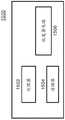
图15示出无线收发器装置1500的示例。装置1500可以用来实现本文中描述的各种技术。装置1500包括处理器1502、存储器1504，该存储器在由处理器执行的计算期间存储处理器可执行指令和数据。装置 1500包括接收和/或发射电路1506，例如，包括用于接收或发射信号和/ 或接收数据或信息位以便通过无线网络传输的射频操作。FIG. 15 shows an example of awireless transceiver apparatus 1500 .Apparatus 1500 may be used to implement various techniques described herein. Theapparatus 1500 includes aprocessor 1502, amemory 1504 that stores processor-executable instructions and data during computations performed by the processor.Apparatus 1500 includes receive and/or transmitcircuitry 1506, eg, including radio frequency operations for receiving or transmitting signals and/or receiving bits of data or information for transmission over a wireless network.

将了解，公开了数据调制的技术，其中可以使用QAM子载波来传输信息信号，而无需使用循环前缀。在一些实施例中，可以使用被称为 OFDM-多载波(MC)的调制技术，其中利用周期脉冲函数来使QAM符号卷积。在一些实施例中，信号的Zak域表示用于使经调制信息信号的带宽和持续时间成形。It will be appreciated that techniques for data modulation are disclosed wherein QAM sub-carriers can be used to transmit information signals without the use of cyclic prefixes. In some embodiments, a modulation technique known as OFDM-Multi-Carrier (MC) may be used in which the QAM symbols are convolved with a periodic impulse function. In some embodiments, the Zak-domain representation of the signal is used to shape the bandwidth and duration of the modulated information signal.

所公开的技术的示例性实现方式Exemplary Implementations of the Disclosed Technology

本文件中描述的所公开的以及其他实施例、模块和功能操作可以在数字电子电路或者计算机软件、固件或硬件中实现，包括本文件中公开的结构和它们的结构等效物或者它们中的一者或多者的组合。所公开的和其他实施例可以被实现为一个或多个计算机程序产品，即，在计算机可读介质上编码的计算机程序指令的一个或多个模块，以便由数据处理装置执行或控制数据处理装置的操作。计算机可读介质可以是机器可读存储设备、机器可读存储基底、存储器设备、影响机器可读传播信号的物质的组成，或者它们中的一者或多者的组合。术语“数据处理装置”涵盖用于处理数据的所有装置、设备和机器，例如，包括可编程处理器、计算机或者多个处理器或计算机。除了硬件之外，装置可以包括为所探讨的计算机程序创建执行环境的代码，例如，构成处理器固件、协议栈、数据库管理系统、操作系统或者它们中的一者或多者的组合的代码。传播信号是人工生成的信号，例如，机器生成的电信号、光信号或电磁信号，所述信号被生成以对信息进行编码以便发射到合适的接收器装置。The disclosed and other embodiments, modules and functional operations described in this document can be implemented in digital electronic circuitry or in computer software, firmware or hardware, including the structures disclosed in this document and their structural equivalents or in A combination of one or more. The disclosed and other embodiments can be implemented as one or more computer program products, i.e., one or more modules of computer program instructions encoded on a computer readable medium for execution by or to control a data processing apparatus operation. The computer-readable medium can be a machine-readable storage device, a machine-readable storage substrate, a memory device, a composition of matter that affects a machine-readable propagated signal, or a combination of one or more thereof. The term "data processing apparatus" encompasses all apparatus, devices, and machines for processing data, including, for example, a programmable processor, a computer, or multiple processors or computers. In addition to hardware, an apparatus may include code that creates an execution environment for the computer program in question, eg, code that constitutes processor firmware, protocol stacks, database management systems, operating systems, or a combination of one or more of these. A propagated signal is an artificially generated signal, eg, a machine-generated electrical, optical or electromagnetic signal, that is generated to encode information for transmission to a suitable receiver device.

计算机程序(也被称为程序、软件、软件应用、脚本或代码)可以用任何形式的编程语言编写，包括编译或解释语言，并且它可以按任何形式部署，包括作为独立程序或模块、部件、子例程，或者适用于计算环境的其他单元。计算机程序不必对应于文件系统中的文件。程序可以存储在保存其他程序或数据的文件的一部分中(例如，存储在标记语言文档中的一个或多个脚本)，存储在专用于所讨论的程序的单个文件中，或者存储在多个协调文件中(例如，存储一个或多个模块、子程序或代码部分的文件)。计算机程序可以部署为在一台计算机上执行，或者在位于一个站点或分布在多个站点之间并通过通信网络互连的多台计算机上执行。A computer program (also known as a program, software, software application, script, or code) may be written in any form of programming language, including compiled or interpreted languages, and it may be deployed in any form, including as a stand-alone program or module, component, Subroutines, or other units applicable to the computing environment. Computer programs do not necessarily correspond to files in the file system. Programs may be stored in part of a file that holds other programs or data (for example, one or more scripts stored in a markup language document), in a single file dedicated to the program in question, or in multiple coordinators. in a file (eg, a file that stores one or more modules, subroutines, or sections of code). A computer program can be deployed to be executed on one computer or on multiple computers located at one site or distributed among multiple sites and interconnected by a communication network.

本文件中描述的过程和逻辑流程可以由一个或多个可编程处理器执行，所述可编程处理器通过在输入数据上操作并且生成输出来执行一个或多个计算机程序以执行功能。过程和逻辑流程也可以由专用逻辑电路执行，并且装置也可以实现为专用逻辑电路，例如，FPGA(现场可编程门阵列)或ASIC(专用集成电路)。The processes and logic flows described in this document can be performed by one or more programmable processors executing one or more computer programs to perform functions by operating on input data and generating output. The processes and logic flows can also be performed by, and apparatus can also be implemented as, special purpose logic circuitry, eg, an FPGA (field programmable gate array) or an ASIC (application specific integrated circuit).

适用于执行计算机程序的处理器包括例如通用和专用微处理器，以及任何种类的数字计算机的任何一个或多个处理器。通常，处理器将从只读存储器或随机存取存储器或两者接收指令和数据。计算机的基本元件是用于执行指令的处理器以及用于存储指令和数据的一个或多个存储器设备。通常，计算机还将包括用于存储数据的一个或多个大容量存储设备，例如磁盘、磁光盘或光盘，或者操作地耦合以从其接收数据或将数据传送到其或这两者。然而，计算机不需要具有此类设备。适用于存储计算机程序指令和数据的计算机可读介质包括所有形式的非易失性存储器、介质和存储器设备，包括例如半导体存储器设备，例如，EPROM、 EEPROM以及闪存设备；磁盘，例如，内部硬盘或可移动盘；磁光盘；以及CD-ROM和DVD-ROM盘。处理器和存储器可以由专用逻辑电路补充或者并入专用逻辑电路中。Processors suitable for the execution of a computer program include, by way of example, both general and special purpose microprocessors, and any one or more processors of any kind of digital computer. Typically, a processor will receive instructions and data from read-only memory or random access memory, or both. The essential elements of a computer are a processor for executing instructions and one or more memory devices for storing instructions and data. Typically, a computer will also include, or be operatively coupled to receive data from, transfer data to, or both, one or more mass storage devices, such as magnetic, magneto-optical or optical disks, for storing data. However, a computer need not have such a device. Computer readable media suitable for storage of computer program instructions and data include all forms of non-volatile memory, media, and memory devices, including, for example, semiconductor memory devices, such as EPROM, EEPROM, and flash memory devices; magnetic disks, such as internal hard disks or Removable disks; magneto-optical disks; and CD-ROM and DVD-ROM disks. The processor and memory may be supplemented by or incorporated in special purpose logic circuitry.

尽管本专利文件含有很多具体方面，但这些不应被解释为限制所要求保护的发明或可以要求保护的内容的范围，而是描述专用于特定实施例的特征。在单独的实施例的上下文中在本文件中描述的某些特征也可以在单个实施例中组合实现。相反地，在单个实施例的上下文中描述的各种特征也可在多个实施方式中分开实现或以任何合适的子组合实现。此外，尽管特征可以在上文描述为在某些组合中起作用并且甚至如最初要求保护的那样，但在一些情况下，所要求保护的组合中的一个或多个特征可以从组合中删除，并且所要求保护的组合可以指向子组合或子组合的变化。类似地，虽然在附图中按特定顺序描绘操作，但这不应被理解为要求此类操作以所示出的特定顺序或按先后顺序执行，或者执行所有示出的操作以实现期望的结果。Although this patent document contains many specific aspects, these should not be construed as limiting the scope of the claimed invention or what may be claimed, but rather as describing features specific to particular embodiments. Certain features that are described in this document in the context of separate embodiments can also be implemented in combination in a single embodiment. Conversely, various features that are described in the context of a single embodiment can also be implemented in multiple implementations separately or in any suitable subcombination. Furthermore, although features may be described above as functioning in certain combinations and even as originally claimed, in some cases one or more features of the claimed combinations may be omitted from the combinations, And claimed combinations may be directed to subcombinations or variations of subcombinations. Similarly, although operations are depicted in the figures in a particular order, this should not be construed as requiring that such operations be performed in the particular order shown, or sequential order, or that all operations shown be performed to achieve desirable results .

仅公开了一些示例和实现方式。基于公开的内容，可以作出对所描述的示例和实现方式以及其他实现方式的变化、更改和增强。Only some examples and implementations are disclosed. Variations, modifications, and enhancements to the described examples and implementations, as well as other implementations, may be made based on what is disclosed.

Claims (10)

Translated fromChinese

1.一种用于无线通信的方法，其包括：1. A method for wireless communication comprising:从信息信号获得波形，obtain the waveform from the information signal,其中所述波形是滤波信号的Zak变换版本，where the waveform is a Zak-transformed version of the filtered signal,其中所述滤波信号是利用脉冲的离散序列的扭曲卷积版本，where the filtered signal is a warped convolutional version using a discrete sequence of pulses,其中在具有延迟轴和多普勒轴的离散点阵上支持所述离散序列，其中所述延迟轴的密度是N的函数，所述多普勒轴的密度是M的函数，其中N和M是互质奇整数，wherein the discrete sequence is supported on a discrete lattice having a delay axis and a Doppler axis, where the density of the delay axis is a function of N, and the density of the Doppler axis is a function of M, where N and M is a coprime odd integer,其中所述波形的第二模糊度函数是利用脉冲的第一模糊度函数的成形版本，以及wherein the second ambiguity function of the waveform is a shaped version of the first ambiguity function using pulses, and其中所述第一模糊度函数是所述离散序列的模糊度函数；wherein the first ambiguity function is the ambiguity function of the discrete sequence;确定所述第二模糊度函数包括具有原点周围的清洁区域的图钉形状；以及determining that the second ambiguity function includes a pushpin shape with a clean area around an origin; and基于所述确定通过无线信道来传输所述波形。The waveform is transmitted over a wireless channel based on the determination.2.如权利要求1所述的方法，其中所述波形包括均匀的时间功率轮廓。2. The method of claim 1, wherein the waveform comprises a uniform temporal power profile.3.如权利要求1所述的方法，其中所述第一模糊度函数是在所述离散点阵上支持的离散模糊度函数。3. The method of claim 1, wherein the first ambiguity function is a discrete ambiguity function supported on the discrete lattice.4.如权利要求3所述的方法，其中所述第二模糊度函数是连续模糊度函数，并且其中所述脉冲成形是基于在所述离散点阵上局部化的所述脉冲。4. The method of claim 3, wherein the second ambiguity function is a continuous ambiguity function, and wherein the pulse shaping is based on the pulses localized on the discrete lattice.5.一种用于无线通信的方法，其包括：5. A method for wireless communication comprising:将信息信号变换成在离散点阵上支持的离散点阵域信号，其中所述离散点阵包括延迟轴和多普勒轴，其中所述延迟轴的密度是N的函数，所述多普勒轴的密度是M的函数，其中N和M是互质奇整数；Transforming an information signal into a discrete lattice domain signal supported on a discrete lattice, wherein the discrete lattice includes a delay axis and a Doppler axis, where the density of the delay axis is a function of N, the Doppler axis The density of the axis is a function of M, where N and M are coprime odd integers;通过二维滤波过程来使所述离散点阵域信号的带宽和持续时间成形以生成经滤波信息信号；shaping the bandwidth and duration of the discrete lattice domain signal by a two-dimensional filtering process to generate a filtered information signal;使用Zak变换从所述经滤波信息信号生成时域信号；generating a time domain signal from the filtered information signal using a Zak transform;确定所述时域信号的模糊度函数包括具有原点周围的清洁区域的图钉形状；以及determining an ambiguity function of the time domain signal comprising a pushpin shape with a clean area around an origin; and基于所述确定通过无线通信信道来传输所述时域信号。The time domain signal is transmitted over a wireless communication channel based on the determination.6.如权利要求5所述的方法，其中所述二维滤波过程包括利用脉冲的扭曲卷积。6. The method of claim 5, wherein the two-dimensional filtering process comprises twisted convolution with pulses.7.如权利要求6所述的方法，其中所述脉冲是所述二维滤波的每个维度的可分离函数。7. The method of claim 6, wherein the pulses are separable functions of each dimension of the two-dimensional filtering.8.如权利要求5所述的方法，其中所述时域信号包括没有中间循环前缀的经调制信息信号。8. The method of claim 5, wherein the time domain signal comprises a modulated information signal without an intermediate cyclic prefix.9.一种无线通信设备，其包括存储指令的存储器以及处理器，其中所述指令在被所述处理器执行时致使所述处理器实现如权利要求1至8中任一项所述的方法。9. A wireless communication device comprising a memory storing instructions and a processor, wherein the instructions, when executed by the processor, cause the processor to implement the method of any one of claims 1 to 8 .10.一种无线信号传输装置，其包括存储器、处理器和传输电路，所述装置实现如权利要求1至8中任一项所述的方法。10. A wireless signal transmission apparatus comprising a memory, a processor and a transmission circuit, the apparatus implementing the method of any one of claims 1 to 8.

Images