CN108763683B - New WENO format construction method under trigonometric function framework - Google Patents

Abstract

Translated fromChinese

一种三角函数框架下新WENO格式构造方法，一方面，用三角函数多项式构造的加权基本无振荡格式比用代数多项式构造的经典基本无振荡格式更易于模拟波类或高频振荡类问题，在光滑区域可以获得高阶数值精度，在激波和接触间断处保持基本无振荡的性质；另一方面，新的TWENO格式虽然和经典五阶WENO格式用了同样五个点的信息，但能得到更低的全局L¹和L^∞范数截断误差。新的TWENO格式采用的线性权不再需要通过繁冗的数值计算得到最优解，可设为满足和为一的任意正数，相比经典的WENO格式更简便，鲁棒性更强，更易于推广到高维空间。该新型TWENO格式有效地数值模拟了几个经典的欧拉问题，充分验证了有效性。

A new WENO scheme construction method under the framework of trigonometric functions. On the one hand, the weighted basic oscillation-free scheme constructed with trigonometric function polynomials is easier to simulate wave-like or high-frequency oscillation problems than the classical basic oscillation-free scheme constructed with algebraic polynomials. The smooth region can obtain high-order numerical accuracy, and maintains basically no oscillation at the shock wave and contact discontinuity; on the other hand, although the new TWENO scheme uses the same five-point information as the classical fifth-order WENO scheme, it can obtain Lower global L1 and^L∞norm truncation errors. The linear weight adopted by the new TWENO format no longer needs to obtain the optimal solution through tedious numerical calculation, and can be set to any positive number that satisfies the sum of one. Compared with the classic WENO format, it is simpler, more robust, and easier to use. generalized to higher dimensional spaces. The new TWENO scheme effectively numerically simulates several classical Euler problems and fully verifies the effectiveness.

Description

Translated fromChinese

一种三角函数框架下新WENO格式构造方法A new WENO format construction method under the framework of trigonometric functions

技术领域technical field

本发明属于计算流体力学工程技术领域，具体涉及了一种三角函数框架下新WENO格式构造方法。The invention belongs to the technical field of computational fluid dynamics engineering, and particularly relates to a new WENO format construction method under the framework of trigonometric functions.

背景技术Background technique

在工程应用中，流场问题常常出现，比如气体动力系统和浅水建模等。因此，制定解决这类问题的鲁棒的、精确的、高效的数值模拟方法至关重要，也吸引了很多研究者的兴趣。1959年，Godunov为解流场问题提出了一阶精度的数值模拟格式。一阶精度的数值模拟方法在捕捉激波时不会出现非物理的数值振荡但会过度抹平强间断，而往往强间断对问题的后续研究有着重要意义，因此需引进高精度数值计算格式模拟强间断类问题。In engineering applications, flow field problems often arise, such as gas dynamic systems and shallow water modeling. Therefore, it is crucial to develop robust, accurate, and efficient numerical simulation methods to solve such problems, which has attracted the interest of many researchers. In 1959, Godunov proposed a numerical simulation format with first-order accuracy for solving flow field problems. The numerical simulation method with first-order accuracy will not cause non-physical numerical oscillations when capturing shock waves, but will overly smooth out strong discontinuities, which are often of great significance to the follow-up research of the problem. Therefore, it is necessary to introduce high-precision numerical calculation formats for simulation. Strong discontinuity problem.

为了提高格式的精度，模拟解的结构以及准确的捕捉激波位置，Harten于1983年首次提出了TVD(Total Variation Diminishing)格式，并在此基础上与Osher于1987年提出了ENO(Essentially Non-Oscillatory)高精度格式。ENO格式的主要思想是在逐次扩展的模板中选用最光滑的模板构造多项式求出单元边界处的值，进而在光滑区域达到高阶精度、高分辨率，同时在间断附近实现基本无振荡的效果。但是，在方法的实现过程中，ENO格式最终只选用所有候选模板中最优的模板，造成计算结果的浪费，且构造的精度越高浪费的越多，导致计算效率不高。因此，Liu，Osher和Chan等于1994年提出了WENO(WeightedEssentially Non-oscillatory)格式，提高了计算结果的利用率并且使得r阶精度的ENO格式提高到r+1阶精度。1996年，Jiang和Shu进一步改善了WENO格式，使得数值精度能够提高到2r-1阶，并设计出新光滑因子和非线性权的构造框架。WENO格式的主要思想是通过低阶重构通量的线性凸组合获得高阶近似。但该经典WENO格式的实现过程中，线性权依赖于母模板，且其求解过程相当复杂，因此，2016年Zhu和Qiu改善了该WENO格式，在维持精度不减的情况下，随机选取大于零且总和为一的线性权。这些格式已被成功地用到很多应用领域，特别是包含激波和复杂解结构的问题，比如模拟可压缩湍流系统和空气声学系统等。In order to improve the accuracy of the format, simulate the structure of the solution and accurately capture the shock position, Harten first proposed the TVD (Total Variation Diminishing) format in 1983, and on this basis, together with Osher in 1987, proposed the ENO (Essentially Non- Oscillatory) high-precision format. The main idea of the ENO format is to select the smoothest template to construct the polynomial in the successively expanded templates to obtain the value at the element boundary, and then achieve high-order precision and high resolution in the smooth region, and at the same time achieve the effect of basically no oscillation near the discontinuity. . However, in the implementation process of the method, the ENO format finally only selects the optimal template among all the candidate templates, resulting in waste of calculation results, and the higher the construction accuracy, the more waste, resulting in low calculation efficiency. Therefore, Liu, Osher and Chan proposed the WENO (Weighted Essentially Non-oscillatory) format in 1994, which improved the utilization of the calculation results and made the r-order precision ENO format improved to r+1-order precision. In 1996, Jiang and Shu further improved the WENO scheme, so that the numerical accuracy can be increased to 2r-1 order, and designed a new smoothing factor and a construction framework for nonlinear weights. The main idea of the WENO scheme is to obtain a high-order approximation by a linear convex combination of the low-order reconstruction fluxes. However, in the implementation process of the classic WENO format, the linear weights depend on the master template, and the solution process is quite complicated. Therefore, in 2016, Zhu and Qiu improved the WENO format. While maintaining the accuracy, the random selection is greater than zero. and a linear weight that sums to one. These formats have been successfully used in many applications, especially problems involving shock waves and complex solution structures, such as modeling compressible turbulent systems and aeroacoustic systems.

波类和高频振荡类问题在工程应用中常常出现。然而，对模拟此类问题的更适合的三角函数多项式插值WENO格式的研究较少。虽然Baron于1976年研究三角函数插值呈现了Neville类方法，Muhlbach提出了牛顿三角函数插值，但是这些成果不能直接应用于ENO类插值格式。为此，Christofi于1996年提出了能直接用于ENO格式中的三角函数重构方法。Zhu和Qiu于2010年提出了用三角函数多项式重构WENO格式的方法，但计算复杂，不易实现。Wave-like and high-frequency oscillation problems often arise in engineering applications. However, less research has been done on the more suitable trigonometric polynomial interpolation WENO scheme for simulating such problems. Although Baron studied trigonometric function interpolation in 1976 and presented Neville-like methods, and Muhlbach proposed Newton's trigonometric function interpolation, these results cannot be directly applied to ENO-like interpolation formats. To this end, Christofi in 1996 proposed a trigonometric function reconstruction method that can be directly used in the ENO format. Zhu and Qiu in 2010 proposed a method to reconstruct the WENO format with trigonometric function polynomials, but the calculation is complex and difficult to implement.

发明内容SUMMARY OF THE INVENTION

本发明针对现有技术中的不足，提供一种三角函数框架下新WENO格式构造方法，能针对各种可压流场问题，进行高精度数值模拟。Aiming at the deficiencies in the prior art, the present invention provides a new WENO format construction method under the framework of trigonometric functions, which can perform high-precision numerical simulation for various compressible flow field problems.

为实现上述目的，本发明采用以下技术方案：To achieve the above object, the present invention adopts the following technical solutions:

一种三角函数框架下新WENO格式构造方法，在笛卡尔坐标系下，利用TWENO格式对可压流场问题进行数值模拟，其特征在于，包括以下步骤：A new WENO format construction method under the framework of trigonometric functions, in the Cartesian coordinate system, using the TWENO format to carry out numerical simulation of the compressible flow field problem, characterized in that the following steps are included:

步骤一、把双曲守恒律方程离散为空间半离散的有限差分格式，采用TWENO格式重构通量的近似值；Step 1. Discrete the hyperbolic conservation law equation into a spatially semi-discrete finite difference format, and use the TWENO format to reconstruct the approximate value of the flux;

步骤二、对控制方程中的时间导数使用三阶TVD Runge-Kutta离散公式将半离散有限差分格式离散成时空全离散有限差分格式；Step 2, using the third-order TVD Runge-Kutta discrete formula to discretize the semi-discrete finite-difference format into a space-time fully discrete finite-difference format for the time derivative in the control equation;

步骤三、根据时空全离散有限差分格式得到下一时间层上的近似值，依次迭代，得到计算区域内终止时刻流场的数值模拟值。Step 3: Obtain the approximate value on the next time layer according to the space-time fully discrete finite difference format, and iterate in turn to obtain the numerical simulation value of the flow field at the termination time in the calculation area.

为优化上述技术方案，采取的具体措施还包括：In order to optimize the above technical solutions, the specific measures taken also include:

所述步骤一中，双曲守恒律方程为：In thestep 1, the hyperbolic conservation law equation is:

其半离散格式的形式为：Its semi-discrete format is of the form:

其中，U＝(ρ,ρu,E)^T表示守恒变量，f(U)＝(ρu,ρu²+p,u(E+p))^T表示通量，U_t表示U对t求导，f(U)_x表示f(U)对x求导，t表示时间变量，x表示空间变量，ρ、u、p、E分别表示流体密度、速度、压强、能量，T表示转置，U₀表示初始状态值，L(U)表示-f(U)_x的空间离散形式；Among them, U=(ρ,ρu,E)^T is the conserved variable, f(U)=(ρu,ρu² +p,u(E+p))^T is the flux, U_t is the derivation of U with respect to t, f(U)_x represents the derivative of f(U) with respect to x, t represents the time variable, x represents the space variable, ρ, u, p, and E represent the fluid density, velocity, pressure, and energy, respectively, T represents the transposition, U₀ Represents the initial state value, L(U) represents the spatial discrete form of -f(U)_x ;

把空间离散成统一长度的网格单元

单元长度

单元中心为

其中i为坐标序号，有：Discretize space into grid cells of uniform length

unit length

The unit center is

Where i is the coordinate number, there are:

其中，

和

分别表示通量f(U)在目标网格单元I_i的边界

和

处的五阶近似的数值通量，U_i(t)表示U在目标网格单元I_i内点x_i处的值U(x_i,t)。in,

and

respectively represent the flux f(U) at the boundary of the target grid cell I_i

and

The numerical flux of the fifth-order approximation at , U_i (t) represents the value U(_xi ,t) of U at point x_i in the target grid cell I_i .

所述步骤一中，求通量f(U)在目标网格单元I_i的边界

和

处的五阶近似值

和

具体步骤如下：In thestep 1, find the boundary of the flux f(U) at the target grid cell I_i

and

fifth-order approximation at

and

Specific steps are as follows:

步骤1、采用Lax-Friedrichs分裂把通量分裂为

其中，

Step 1. Use Lax-Friedrichs splitting to split the flux into

in,

步骤2、将目标网格单元I_i以及其周围共五个网格单元组成一个大模板T₁＝[I_i-2,I_i-1,I_i,I_i+1,I_i+2]，从大模板中选择两个包含两个单元的小模板T₂＝[I_i-1,I_i]和T₃＝[I_i,I_i+1]；Step 2. Form a large template T₁ =[I_i-2 ,I_i-1 ,I_i ,I_i+1 ,I_i+2 ] with the target grid unit I_i and its surrounding five grid units , select two small templates containing two units T₂ =[I_i-1 ,I_i ] and T₃ =[I_i ,I_i+1 ] from the large template;

步骤3、在T₁、T₂、T₃每个模板上分别重构三角函数多项式p₁(x)、p₂(x)和p₃(x)，使得：Step 3. Reconstruct the trigonometric function polynomials p₁ (x), p₂ (x) and p₃ (x) on each template of T₁ , T₂ , and T₃ respectively, so that:

p₂(x),p₃(x)∈span{1,sin(x-x_i)}；p₂ (x),p₃ (x)∈span{1,sin(xx_i )};

步骤4、任意取三组线性权：Step 4. Arbitrarily take three sets of linear weights:

γ₁＝0.98，γ₂＝0.01，γ₃＝0.01；γ₁ =0.98, γ₂ =0.01, γ₃ =0.01;

γ₁＝1/3，γ₂＝1/3，γ₃＝1/3；γ₁ =1/3, γ₂ =1/3, γ₃ =1/3;

γ₁＝0.01，γ₂＝0.495，γ₃＝0.495；γ₁ =0.01, γ₂ =0.495, γ₃ =0.495;

步骤5、计算光滑指示器β_l，用于衡量重构多项式p_l(x)在目标单元上的光滑度，计算公式为：Step 5. Calculate the smoothness indicator β_l , which is used to measure the smoothness of the reconstructed polynomial p_l (x) on the target unit. The calculation formula is:

其中，l＝1,2,3表示对应模板序号，

表示多项式p_l(x)对x的α阶导数，r₁＝4，r₂＝1，r₃＝1；Among them, l=1,2,3 represents the corresponding template serial number,

represents the α-order derivative of the polynomial p_l (x) with respect to x, r₁ =4, r₂ =1, r₃ =1;

步骤6、通过线性权γ_l和光滑指示器β_l计算非线性权ω_l，其计算公式为：Step 6. Calculate the nonlinear weight ω_l through the linear weight γ_l and the smooth indicator β_l , and the calculation formula is:

其中，

τ为计算过程中的过渡值，ε＝10^-6；in,

τ is the transition value in the calculation process, ε=10⁻⁶ ;

步骤7、求出数值通量分裂f⁺(U)在点

处的TWENO重构值：Step 7. Find the numerical flux split f⁺ (U) at the point

The reconstructed value of TWENO at:

同理，求出数值通量分裂f^-(U)在点

处的TWENO重构值、数值通量分裂f⁺(U)在点

处的TWENO重构值、数值通量分裂f^-(U)在点

处的TWENO重构值；Similarly, find the numerical flux split f^- (U) at the point

TWENO reconstruction value at , numerical flux split f⁺ (U) at point

TWENO reconstruction value at , numerical flux split f^- (U) at point

The reconstructed value of TWENO at ;

将计算结果代入含有时间导数项的半离散有限差分格式，得到关于时间导数的常微分方程。Substitute the calculation result into the semi-discrete finite difference scheme containing the time derivative term, and obtain the ordinary differential equation about the time derivative.

所述步骤3中，具体步骤如下：In thestep 3, the specific steps are as follows:

步骤3.1、在三个模板T₁、T₂和T₃上分别构造三角函数多项式p₁(x)、p₂(x)和p₃(x)，使其满足:Step 3.1. Construct trigonometric function polynomials p₁ (x), p₂ (x) and p₃ (x) on the three templates T₁ , T₂ and T₃ respectively, so that they satisfy:

步骤3.2、得到每个模板上的三角函数插值多项式p₁(x)、p₂(x)和p₃(x)，如下：Step 3.2. Obtain the trigonometric function interpolation polynomials p₁ (x), p₂ (x) and p₃ (x) on each template, as follows:

其中，I_i-2、I_i-1、I_i、I_i+1、I_i+2分别表示第i-2、i-1、i、i+1、i+2个网格单元，

f_i⁺、

分别表示f⁺(U)在点x_i-2、x_i-1、x_i、x_i+1、x_i+2的值。Among them, I_i-2 , I_i-1 , I_i , I_i+1 , and I_i+2 represent the i-2, i-1, i, i+1, and i+2 grid cells, respectively,

f_i⁺ ,

represent the values of f⁺ (U) at points x_i-2 , x_i-1 , x_i , x_i+1 , and x_i+2 , respectively.

所述步骤二中，利用三阶TVD Runge-Kutta离散公式：In thestep 2, the third-order TVD Runge-Kutta discrete formula is used:

得到时空全离散有限差分格式，其中，U⁽¹⁾,U⁽²⁾为中间过渡值，Δt为时间步长，上标n表示第n时间层，L(Uⁿ),L(U⁽¹⁾),L(U⁽²⁾)为-f(U)_x的高阶空间离散形式的近似值。The space-time fully discrete finite difference scheme is obtained, where U⁽¹⁾ , U⁽²⁾ are intermediate transition values, Δt is the time step, the superscript n represents the nth time layer, L(Uⁿ ), L(U^{(1 )} ), L(U⁽²⁾ ) is an approximation of the higher-order spatial discrete form of -f(U)_x .

所述步骤三中，时空全离散有限差分格式为关于时间层的迭代公式，初始状态值已知，通过迭代公式求出下一时间层的近似值，依次得到终止时刻计算区域内的数值模拟值。In the third step, the space-time fully discrete finite difference format is an iterative formula about the time layer, the initial state value is known, the approximate value of the next time layer is obtained through the iterative formula, and the numerical simulation value in the calculation area at the termination time is sequentially obtained.

本发明的有益效果是：相比于WENO格式，该TWENO格式通过把三角函数多项式而不是代数多项式作为有限差分TWENO格式的构建模块，模拟了波类和高频振荡类可压流场问题，同时在光滑区域能够达到高阶精度；相比于已有三角函数多项式重构格式，该TWENO格式得到的全局L¹截断误差与L^∞截断误差更小，同时也避免了在强激波和接触间断处产生非物理振荡，该新五阶TWENO格式中的相关线性权不再需要通过复杂的计算得到而是被设为和为一的任意正数，因此该新TWENO格式具有更简便更易拓展到高维空间的优势。The beneficial effects of the present invention are: compared with the WENO format, the TWENO format uses trigonometric function polynomials instead of algebraic polynomials as the building blocks of the finite-difference TWENO format to simulate the wave-like and high-frequency oscillation-like compressible flow field problems, and simultaneously High-order accuracy can be achieved in smooth regions; compared with the existing trigonometric function polynomial reconstruction schemes, the global L¹ truncation error and L^∞ truncation error obtained by the TWENO scheme are smaller, and it also avoids strong shock waves and contact discontinuities. where non-physical oscillations are generated, the relevant linear weights in the new fifth-order TWENO scheme no longer need to be obtained through complex calculations, but are set to any positive number whose sum is one, so the new TWENO scheme is simpler and easier to extend to high The advantage of dimensional space.

附图说明Description of drawings

图1a-1c是实施例一中的台阶问题，利用本发明的有限差分TWENO格式得到的密度等值线图，分别采用线性权①、②、③。Figures 1a-1c show the step problem in the first embodiment. The density contour map obtained by using the finite difference TWENO format of the present invention adoptslinear weights ①, ②, and ③ respectively.

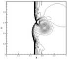
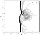
图2a-2c是实施例二中的双马赫问题，利用本发明的有限差分TWENO格式得到的密度等值线图，分别采用线性权①、②、③。Figures 2a-2c are the double Mach problem in the second embodiment. The density contour map obtained by using the finite difference TWENO format of the present invention adoptslinear weights ①, ②, and ③ respectively.

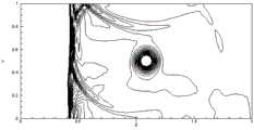
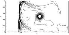
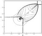
图3a-3c是实施例三中的激波和涡流相互干扰问题，利用本发明的有限差分TWENO格式得到的t＝0.35时的压强等值线图，分别采用线性权①、②、③。Figures 3a-3c are the problem of mutual interference between shock waves and eddy currents in the third embodiment. The pressure contour diagrams at t=0.35 are obtained by using the finite difference TWENO format of the present invention, andlinear weights ①, ②, and ③ are used respectively.

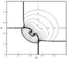
图4a-4c是实施例三中的激波和涡流相互干扰问题，利用本发明的有限差分TWENO格式得到的t＝0.6时的压强等值线图，分别采用线性权①、②、③。Figures 4a-4c illustrate the mutual interference problem between shock waves and eddy currents in the third embodiment. The pressure contour diagrams at t=0.6 are obtained by using the finite difference TWENO format of the present invention, usinglinear weights ①, ②, and ③ respectively.

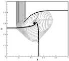
图5a-5c是实施例三中的激波和涡流相互干扰问题，利用本发明的有限差分TWENO格式得到的t＝0.8时的压强等值线图，分别采用线性权①、②、③。Figures 5a-5c are the problem of mutual interference between shock waves and eddy currents in the third embodiment. The pressure contour diagrams at t=0.8 are obtained by using the finite difference TWENO format of the present invention, andlinear weights ①, ②, and ③ are used respectively.

图6a-6c是实施例四中初值条件为(19)的二维Euler黎曼问题，利用本发明的有限差分TWENO格式得到的t＝0.25时的密度等值线图，分别采用线性权①、②、③。Figures 6a-6c are the two-dimensional Euler Riemann problem with the initial value condition (19) in the fourth embodiment, and the density contour plots at t=0.25 obtained by using the finite difference TWENO format of the present invention, respectively using linear weights① , ②, ③.

图7a-7c是实施例四中初值条件为(20)的二维Euler黎曼问题，利用本发明的有限差分TWENO格式得到的t＝0.25时的密度等值线图，分别采用线性权①、②、③。Figures 7a-7c are the two-dimensional Euler Riemann problem with the initial value condition (20) in the fourth embodiment, and the density contour plots at t=0.25 obtained by using the finite difference TWENO format of the present invention, respectively adopting linear weights① , ②, ③.

图8a-8c是实施例四中初值条件为(21)的二维Euler黎曼问题，利用本发明的有限差分TWENO格式得到的t＝0.3时的密度等值线图，分别采用线性权①、②、③。Figures 8a-8c are the two-dimensional Euler Riemann problem with the initial value condition (21) in the fourth embodiment, and the density contour plots at t=0.3 obtained by using the finite difference TWENO format of the present invention, respectively using linear weights① , ②, ③.

图9a-9c是实施例四中初值条件为(22)的二维Euler黎曼问题，利用本发明的有限差分TWENO格式得到的t＝0.2时的密度等值线图，分别采用线性权①、②、③。Figures 9a-9c are the two-dimensional Euler Riemann problem with the initial value condition (22) in the fourth embodiment, and the density contour plots at t=0.2 obtained by using the finite difference TWENO format of the present invention, respectively adopting linear weights① , ②, ③.

图10a-10c是实施例四中初值条件为(23)的二维Euler黎曼问题，利用本发明的有限差分TWENO格式得到的t＝0.3时的密度等值线图，分别采用线性权①、②、③。Figures 10a-10c are the two-dimensional Euler Riemann problem with the initial value condition (23) in the fourth embodiment, and the density contour plots at t=0.3 obtained by using the finite difference TWENO format of the present invention, respectively using linear weights① , ②, ③.

具体实施方式Detailed ways

现在结合附图对本发明作进一步详细的说明。The present invention will now be described in further detail with reference to the accompanying drawings.

本发明给出了笛卡尔网格下解可压流场问题的新型五阶有限差分TWENO高精度数值计算格式的构造过程，相比于经典WENO格式，该TWENO格式通过把重构的三角函数多项式而不是重构的代数多项式作为有限差分WENO格式的构建模块，解决了波类和高频振荡类的可压流场问题的数值模拟，且在光滑区域能够达到高阶精度近似，捕捉到尖锐和无振荡激波的转换。新的TWENO格式采用的线性权不再需要通过繁冗的数值计算得到，可设为满足和为一的任意正数，此格式方法简单、精度高，易于推广到多维空间中。该方法在笛卡尔坐标系下，利用TWENO格式对可压流场问题进行数值模拟，具体步骤如下：The invention provides the construction process of a new fifth-order finite difference TWENO high-precision numerical calculation format for solving the compressible flow field problem under Cartesian grid. The non-reconstructed algebraic polynomial is used as the building block of the finite-difference WENO format to solve the numerical simulation of compressible flow field problems of the wave type and high-frequency oscillation type, and can achieve high-order precision approximation in the smooth region, capturing sharp and non-linear Conversion of oscillatory shock waves. The linear weight adopted by the new TWENO format no longer needs to be obtained by tedious numerical calculation, and can be set to any positive number satisfying the sum of one. This method uses the TWENO format to numerically simulate the compressible flow field problem in the Cartesian coordinate system. The specific steps are as follows:

一、把双曲守恒律方程离散为空间半离散的有限差分格式，采用TWENO格式重构通量的近似值。1. Discrete the hyperbolic conservation law equation into a spatially semi-discrete finite difference scheme, and use the TWENO scheme to reconstruct the approximate value of the flux.

考虑一维双曲守恒律方程：Consider the one-dimensional hyperbolic conservation law equation:

其半离散格式的形式为：Its semi-discrete format is of the form:

其中，U＝(ρ,ρu,E)^T表示守恒变量，f(U)＝(ρu,ρu²+p,u(E+p))^T表示通量，U_t表示U对t求导，f(U)_x表示f(U)对x求导，t表示时间变量，x表示空间变量，ρ、u、p、E分别表示流体密度、速度、压强、能量，T表示转置，U₀表示初始状态值，L(U)表示-f(U)_x的空间离散形式。Among them, U=(ρ,ρu,E)^T is the conserved variable, f(U)=(ρu,ρu² +p,u(E+p))^T is the flux, U_t is the derivation of U with respect to t, f(U)_x represents the derivative of f(U) with respect to x, t represents the time variable, x represents the space variable, ρ, u, p, and E represent the fluid density, velocity, pressure, and energy, respectively, T represents the transposition, U₀ represents the initial state value, and L(U) represents the spatially discrete form of -f(U)_x .

把空间离散成统一长度的网格单元

单元长度

单元中心为

其中i为坐标序号，有：Discretize space into grid cells of uniform length

unit length

The unit center is

Where i is the coordinate number, there are:

其中，

和

分别表示通量f(U)在目标单元I_i的边界

和

处的五阶近似的数值通量，U_i(t)表示U在网格单元I_i内点x_i处的值U(x_i,t)。in,

and

respectively represent the flux f(U) at the boundary of the target cell I_i

and

The numerical flux of the fifth-order approximation at , U_i (t) represents the value U(_xi ,t) of U at point x_i in grid cell I_i .

求通量f(U)在目标单元I_i的边界

和

处的五阶近似值

和

具体步骤如下：Find the flux f(U) at the boundary of the target cell I_i

and

fifth-order approximation at

and

Specific steps are as follows:

步骤1、用最简单的Lax-Friedrichs分裂把通量分裂为

其中

为了简单起见，本发明只描述f⁺(U)在点

处的重构过程并将其定义为

Step 1. Use the simplest Lax-Friedrichs split to split the flux into

in

For simplicity, the present invention only describes f⁺ (U) at the point

the refactoring process at and define it as

步骤2、将目标单元I_i以及其周围共5个网格单元组成一个大模板T₁＝[I_i-2,I_i-1,I_i,I_i+1,I_i+2]，从大模板中选择两个包含两个单元的小模板T₂＝[I_i-1,I_i]和T₃＝[I_i,I_i+1]，其中I_i为对应序号的网格单元。Step 2. Form a large template T₁ =[I_i-2 , I_i-1 , I_i , I_i+1 , I_i+2 ] from the target unit I_i and its surrounding 5 grid units, from In the large template, two small templates containing two cells are selected, T₂ =[I_i-1 , I_i ] and T₃ =[I_i , I_i+1 ], where I_i is a grid cell with a corresponding serial number.

步骤3、在每个模板上分别重构三角函数多项式p₁(x)、p₂(x)和p₃(x)，使得：Step 3. Reconstruct the trigonometric function polynomials p₁ (x), p₂ (x) and p₃ (x) on each template respectively, so that:

p₂(x),p₃(x)∈span{1,sin(x-x_i)}。p₂ (x),p₃ (x)∈span{1,sin(xx_i )}.

其具体过程如下：The specific process is as follows:

步骤3.1、在三个模板T₁、T₂和T₃上分别构造三角函数多项式p₁(x)、p₂(x)和p₃(x)，使其满足:Step 3.1. Construct trigonometric function polynomials p₁ (x), p₂ (x) and p₃ (x) on the three templates T₁ , T₂ and T₃ respectively, so that they satisfy:

步骤3.2、得到每个模板上的三角函数插值多项式p₁(x)、p₂(x)和p₃(x)，如下：Step 3.2. Obtain the trigonometric function interpolation polynomials p₁ (x), p₂ (x) and p₃ (x) on each template, as follows:

其中，I_i-2、I_i-1、I_i、I_i+1、I_i+2分别表示第i-2、i-1、i、i+1、i+2个单元，

f_i⁺、

分别表示f⁺(U)在点x_i-2、x_i-1、x_i、x_i+1、x_i+2的值，h为网格步长。Wherein, I_i-2 , I_i-1 , I_i , I_i+1 , and I_i+2 represent the i-2, i-1, i, i+1, and i+2 units, respectively,

f_i⁺ ,

respectively represent the values of f⁺ (U) at points x_i-2 , x_i-1 , x_i , x_i+1 , and x_i+2 , and h is the grid step size.

步骤4、任意取三组线性权：Step 4. Arbitrarily take three sets of linear weights:

①γ₁＝0.98，γ₂＝0.01，γ₃＝0.01；①γ₁ =0.98, γ₂ =0.01, γ₃ =0.01;

②γ₁＝1/3，γ₂＝1/3，γ₃＝1/3；②γ₁ =1/3, γ₂ =1/3, γ₃ =1/3;

③γ₁＝0.01，γ₂＝0.495，γ₃＝0.495。③ γ₁ =0.01, γ₂ =0.495, γ₃ =0.495.

步骤5、计算光滑指示器β_l，用于衡量重构多项式p_l(x)在目标单元上的光滑度，计算公式为：Step 5. Calculate the smoothness indicator β_l , which is used to measure the smoothness of the reconstructed polynomial p_l (x) on the target unit. The calculation formula is:

其中，l＝1,2,3表示对应模板序号，

表示多项式p_l(x)对x的α阶导数，r₁＝4，r₂＝1，r₃＝1。Among them, l=1,2,3 represents the corresponding template serial number,

Represents the alpha derivative of the polynomial p_l (x) with respect to x, where r₁ =4, r₂ =1, and r₃ =1.

步骤6、通过线性权γ_l和光滑指示器β_l计算非线性权ω_l，其计算公式为：Step 6. Calculate the nonlinear weight ω_l through the linear weight γ_l and the smooth indicator β_l , and the calculation formula is:

其中，l＝1,2,3表示对应模板序号，

τ为计算过程中的过渡值，β_l为光滑指示器，ε＝10^-6防止分母为零。Among them, l=1,2,3 represents the corresponding template serial number,

τ is the transition value in the calculation process, β_l is the smoothness indicator, and ε=10⁻⁶ prevents the denominator from being zero.

步骤7、求出数值通量分裂f⁺(U)在点

处的TWENO重构值：Step 7. Find the numerical flux split f⁺ (U) at the point

The reconstructed value of TWENO at:

其次，将计算结果代入含有时间导数项的半离散有限差分格式，得到关于时间导数的常微分方程。Secondly, the calculation result is substituted into the semi-discrete finite difference scheme containing the time derivative term, and the ordinary differential equation about the time derivative is obtained.

二、对控制方程中的时间导数使用三阶TVD Runge-Kutta离散公式将半离散有限差分格式离散成时空全离散有限差分格式。2. Using the third-order TVD Runge-Kutta discrete formula to discretize the semi-discrete finite-difference format into a space-time fully discrete finite-difference format for the time derivative in the control equation.

利用三阶TVD Runge-Kutta离散公式：Using the third-order TVD Runge-Kutta discrete formula:

得到时空全离散有限差分格式，其中，U⁽¹⁾,U⁽²⁾为中间过渡值，Δt为时间步长，上标n表示第n时间层，L(Uⁿ),L(U⁽¹⁾),L(U⁽²⁾)为-f(U)_x的高阶空间离散形式的近似值。The space-time fully discrete finite difference scheme is obtained, where U⁽¹⁾ , U⁽²⁾ are intermediate transition values, Δt is the time step, the superscript n represents the nth time layer, L(Uⁿ ), L(U^{(1 )} ), L(U⁽²⁾ ) is an approximation of the higher-order spatial discrete form of -f(U)_x .

三、根据时空全离散有限差分格式得到下一时间层上的近似值，依次迭代，得到计算区域内终止时刻流场的数值模拟值。3. Obtain the approximate value on the next time layer according to the space-time fully discrete finite difference scheme, and iterate in turn to obtain the numerical simulation value of the flow field at the termination time in the calculation area.

时空全离散有限差分格式为关于时间层的迭代公式，初始状态值已知，通过迭代公式求出下一时间层的近似值，依次得到终止时刻计算区域内的数值模拟值。对于二维问题，逐维用上面的重构过程。The space-time fully discrete finite difference scheme is an iterative formula about the time layer, the initial state value is known, the approximate value of the next time layer is obtained through the iterative formula, and the numerical simulation value in the calculation area at the termination time is obtained in turn. For two-dimensional problems, use the above reconstruction process dimension by dimension.

下面给出几个算例作为本发明所公开方法的具体实施例。Several calculation examples are given below as specific embodiments of the method disclosed in the present invention.

实施例一、台阶问题。该问题是Emery于1968年提出的一个用于检验非线性双曲型守恒律格式的经典算例。初始数据为水平来流马赫数为3，密度为1.4，水平速度为3，竖直速度为0，压强为1，管道区域为[0,3]×[0,1]，在距离左边界0.6处有一高度为0.2的台阶，且台阶延伸到管道的尽头。上下边界为反射边界，左边界为来流边界，右边界为出流边界。图1a-1c给出了t＝4时的密度等值线图。Embodiment 1. Step problem. This problem is a classical example proposed by Emery in 1968 to test the nonlinear hyperbolic conservation law scheme. The initial data is that the horizontal incoming Mach number is 3, the density is 1.4, the horizontal velocity is 3, the vertical velocity is 0, the pressure is 1, the pipeline area is [0,3]×[0,1], at a distance of 0.6 from the left boundary There is a step with a height of 0.2, and the step extends to the end of the pipe. The upper and lower boundaries are the reflection boundaries, the left boundary is the incoming flow boundary, and the right boundary is the outflow boundary. Figures 1a-1c show density contour plots at t=4.

实施例二、双马赫反射问题。该问题描述了一个与x轴成60°角的强激波射到反射墙上发生的变化，来流是马赫数为10的强激波。计算区域为[0,4]×[0,1]。区域底部从

y＝0处开始为反射边界条件，其它的底部边界(从x＝0到

那部分)为波前条件。图2a-2c给出了t＝0.2时在[0,3]×[0,1]区域的密度等值线图。Embodiment 2. Double Mach reflection problem. The problem describes the changes that occur when a strong shock wave hits a reflecting wall at an angle of 60° to the x-axis, and the incoming flow is a strong shock wave with a Mach number of 10. The calculation area is [0,4]×[0,1]. the bottom of the area from

The reflection boundary condition starts at y=0, and the other bottom boundaries (from x=0 to

that part) is the wavefront condition. Figures 2a-2c show density contour plots in the [0,3]×[0,1] region at t=0.2.

实施例三、激波和涡流相互干扰问题。马赫数为1.1的激波位于x＝0.5处且垂直于x轴。激波初始状态是

小涡流位于该激波的左边且其中心位于(x_c,y_c)＝(0.25,0.5)处。涡流可看成平均流的速度，温度和熵的扰动，表示为：Embodiment 3. The problem of mutual interference between shock waves and eddy currents. A shock wave with Mach 1.1 is located at x=0.5 and is perpendicular to the x-axis. The initial state of the shock wave is

A small eddy current is located to the left of the shock and its center is located at (x_c , y_c )=(0.25, 0.5). The eddy current can be regarded as the perturbation of the velocity, temperature and entropy of the mean flow, expressed as:

其中，τ＝r/r_c，

ε＝0.3，r_c＝0.05，α＝0.204，γ＝1.4，计算区域为[0,2]×[0,1]。图3a-3c给出了t＝0.35时在[0,1]×[0,1]区域的压强等值线图。图4a-4c给出了t＝0.6时在[0.4,1.45]×[0,1]区域的压强等值线图。图5a-5c给出了t＝0.8时在[0,2]×[0,1]区域的压强等值线图。where τ=_r /rc ,

ε=0.3,_rc =0.05, α=0.204, γ=1.4, and the calculation area is [0,2]×[0,1]. Figures 3a-3c show the pressure contour plots in the [0,1]×[0,1] region at t=0.35. Figures 4a-4c show the pressure contour plots in the [0.4, 1.45] × [0, 1] region at t=0.6. Figures 5a-5c show the pressure contour plots in the [0,2]×[0,1] region at t=0.8.

实施例四、二维Euler黎曼问题。计算区域为[0,1]×[0,1]，初值条件分别设为：Embodiment 4. Two-dimensional Euler-Riemann problem. The calculation area is [0,1]×[0,1], and the initial value conditions are respectively set as:

图6a-6c给出了初值条件为(18)时二维Euler黎曼问题在t＝0.25时刻的密度等值线图。图7a-7c给出了初值条件为(19)时二维Euler黎曼问题在t＝0.25时刻的密度等值线图。图8a-8c给出了初值条件为(20)时二维Euler黎曼问题在t＝0.3时刻的密度等值线图。图9a-9c给出了初值条件为(21)时二维Euler黎曼问题在t＝0.2时刻的密度等值线图。图10a-10c给出了初值条件为(22)时二维Euler黎曼问题在t＝0.3时刻的密度等值线图。从图中可以看出基于三角函数多项式空间的有限差分TWENO格式对本发明任意取得的线性权都可以很好的捕捉到黎曼问题的大部分流动特性。Figures 6a-6c show the density contour map of the two-dimensional Euler-Riemann problem at t=0.25 when the initial value condition is (18). Figures 7a-7c show the density contour map of the two-dimensional Euler-Riemann problem at t=0.25 when the initial value condition is (19). Figures 8a-8c show the density contour map of the two-dimensional Euler-Riemann problem at t=0.3 when the initial value condition is (20). Figures 9a-9c show the density contour map of the two-dimensional Euler-Riemann problem at t=0.2 when the initial value condition is (21). Figures 10a-10c show the density contour plots of the two-dimensional Euler-Riemann problem at t=0.3 when the initial value condition is (22). It can be seen from the figure that the finite difference TWENO scheme based on the trigonometric function polynomial space can well capture most of the flow characteristics of the Riemann problem for any linear weight obtained by the present invention.

以上仅是本发明的优选实施方式，本发明的保护范围并不仅局限于上述实施例，凡属于本发明思路下的技术方案均属于本发明的保护范围。应当指出，对于本技术领域的普通技术人员来说，在不脱离本发明原理前提下的若干改进和润饰，应视为本发明的保护范围。The above are only preferred embodiments of the present invention, and the protection scope of the present invention is not limited to the above-mentioned embodiments, and all technical solutions that belong to the idea of the present invention belong to the protection scope of the present invention. It should be pointed out that for those skilled in the art, some improvements and modifications without departing from the principle of the present invention should be regarded as the protection scope of the present invention.

Claims (4)

1. A new WENO format construction method under a trigonometric function frame is characterized in that a TWENO format is utilized to carry out numerical simulation on a compressible flow field problem under a Cartesian coordinate system, and the method comprises the following steps:

dispersing a hyperbolic conservation law equation into a space semi-discrete finite difference format, and reconstructing an approximate value of flux by adopting a TWENO format;

step two, dispersing the semi-discrete finite difference format into a space-time fully-discrete finite difference format by using a three-order TVD Runge-Kutta discrete formula for the time derivative in the control equation;

obtaining an approximate value on the next time layer according to a space-time full-discrete finite difference format, and sequentially iterating to obtain a numerical simulation value of a flow field at the termination time in a calculation region;

in the first step, the hyperbolic conservation law equation is as follows:

the semi-discrete format is in the form of:

where U ═ p, ρ U, E)^TDenotes a conservation variable, f (u) ═ p u, p u²+p,u(E+p))^TRepresents the flux, U_tMeaning U is derived from t, f (U)_xDenotes f (U) derivation of x, T time variable, x space variable, ρ, U, p, E respectively fluid density, velocity, pressure, energy, T transposition, U₀Denotes an initial state value, L (U) denotes-f (U)_xA spatially discrete form of (a);

discretizing space into grid cells of uniform length

Length of cell

The center of the unit is

Where i is the coordinate number, there are:

wherein,

and

respectively representing the flux f (U) in the target grid cell I_iIs limited by

And

numerical flux of the fifth order approximation, U_i(t) indicates that U is in the target grid cell I_iInner point x_iValue of (x) of_i,t)；

Wherein, the flux f (U) is calculated at the target grid unit I_iIs limited by

And

approximation of the fifth order of

And

the method comprises the following specific steps:

step 1, adopting Lax-Friedrichs splitting to split flux into

Wherein,

step 2, target grid unit I_iAnd a large template T consisting of five grid units around the large template T₁＝[I_i-2,I_i-1,I_i,I_i+1,I_i+2]Selecting two small templates T containing two units from the large template₂＝[I_i-1,I_i]And T₃＝[I_i,I_i+1]；

Step 3, at T₁、T₂、T₃Respectively reconstructing trigonometric function polynomial p on each template₁(x)、p₂(x) And p₃(x) So that:

p₂(x),p₃(x)∈span{1,sin(x-x_i)}；

and 4, arbitrarily taking three groups of linear weights:

γ₁＝0.98，γ₂＝0.01，γ₃＝0.01；

γ₁＝1/3，γ₂＝1/3，γ₃＝1/3；

γ₁＝0.01，γ₂＝0.495，γ₃＝0.495；

step 5, calculating a smooth indicator beta_lFor evaluating the reconstruction polynomial p_l(x) The smoothness on the target cell is calculated by the formula:

wherein, l is 1,2,3 represents corresponding template serial number,

representing a polynomial p_l(x) Derivative of order alpha to x, r₁＝4，r₂＝1，r₃＝1；

Step 6, passing the linear weight gamma_lAnd a smoothness indicator beta_lCalculating the non-linear weight omega_lThe calculation formula is as follows:

wherein,

tau is the transition value in the calculation process, epsilon is 10^-6；

Step 7, solving numerical flux split f⁺(U) at point

TWENO reconstruction value of (a):

analogously, the numerical flux split f is determined^-(U) at point

TWENO reconstruction value, numerical flux split f⁺(U) at point

TWENO reconstruction value, numerical flux split f^-(U) at point

A TWENO reconstruction value of (a);

and substituting the calculation result into a semi-discrete finite difference format containing a time derivative term to obtain an ordinary differential equation related to the time derivative.

2. The method of claim 1, wherein the new WENO format is constructed under a trigonometric function framework: in the step 3, the specific steps are as follows:

step 3.1, three templates T₁、T₂And T₃Respectively constructing a trigonometric function polynomial p₁(x)、p₂(x) And p₃(x) So that it satisfies:

step 3.2, obtaining a trigonometric function polynomial p on each template₁(x)、p₂(x) And p₃(x) The following are:

wherein, I_i-2、I_i-1、I_i、I_i+1、I_i+2Respectively represent the (i-2) th grid unit, the (i-1) th grid unit, the (i + 1) th grid unit and the (i + 2) th grid unit,

respectively represents f⁺(U) at point x_i-2、x_i-1、x_i、x_i+1、x_i+2The value of (c).

3. The method of claim 1, wherein the new WENO format is constructed under a trigonometric function framework: in the second step, a third-order TVD Runge-Kutta discrete formula is utilized:

obtaining a space-time fully discrete finite difference format, wherein U⁽¹⁾,U⁽²⁾For intermediate transition values, Δ t is the time step, and the superscript n denotes the nth time layer, L (U)ⁿ),L(U⁽¹⁾),L(U⁽²⁾) Is-f (U)_xAn approximation of a higher order spatially discrete form of (a).

4. The method of claim 3, wherein the new WENO format under trigonometric function framework is as follows: in the third step, the space-time full-discrete finite difference format is an iterative formula about the time layer, the initial state value is known, the approximate value of the next time layer is calculated through the iterative formula, and the numerical simulation value in the calculation region of the termination time is sequentially obtained.

Images