Chart visualization#
Note
The examples below assume that you’re usingJupyter.
This section demonstrates visualization through charting. For information onvisualization of tabular data please see the section onTable Visualization.
We use the standard convention for referencing the matplotlib API:
In [1]:importmatplotlib.pyplotaspltIn [2]:plt.close("all")
We provide the basics in pandas to easily create decent looking plots.Seethe ecosystem page for visualizationlibraries that go beyond the basics documented here.
Note
All calls tonp.random are seeded with 123456.
Basic plotting:plot#
We will demonstrate the basics, see thecookbook forsome advanced strategies.
Theplot method on Series and DataFrame is just a simple wrapper aroundplt.plot():
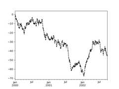
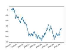
In [3]:np.random.seed(123456)In [4]:ts=pd.Series(np.random.randn(1000),index=pd.date_range("1/1/2000",periods=1000))In [5]:ts=ts.cumsum()In [6]:ts.plot();
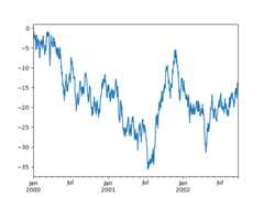
If the index consists of dates, it callsgcf().autofmt_xdate()to try to format the x-axis nicely as per above.
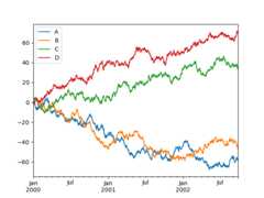
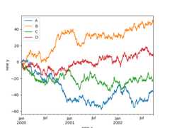
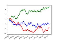
On DataFrame,plot() is a convenience to plot all of the columns with labels:
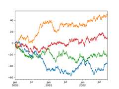
In [7]:df=pd.DataFrame(np.random.randn(1000,4),index=ts.index,columns=list("ABCD"))In [8]:df=df.cumsum()In [9]:plt.figure();In [10]:df.plot();
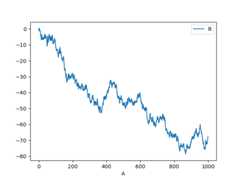
You can plot one column versus another using thex andy keywords inplot():
In [11]:df3=pd.DataFrame(np.random.randn(1000,2),columns=["B","C"]).cumsum()In [12]:df3["A"]=pd.Series(list(range(len(df))))In [13]:df3.plot(x="A",y="B");
Note
For more formatting and styling options, seeformatting below.
Other plots#
Plotting methods allow for a handful of plot styles other than thedefault line plot. These methods can be provided as thekindkeyword argument toplot(), and include:
‘hist’ for histogram
‘box’ for boxplot
‘area’ for area plots
‘scatter’ for scatter plots
‘hexbin’ for hexagonal bin plots
‘pie’ for pie plots
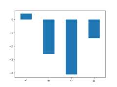
For example, a bar plot can be created the following way:
In [14]:plt.figure();In [15]:df.iloc[5].plot(kind="bar");
You can also create these other plots using the methodsDataFrame.plot.<kind> instead of providing thekind keyword argument. This makes it easier to discover plot methods and the specific arguments they use:
In [16]:df=pd.DataFrame()In [17]:df.plot.<TAB># noqa: E225, E999df.plot.area df.plot.barh df.plot.density df.plot.hist df.plot.line df.plot.scatterdf.plot.bar df.plot.box df.plot.hexbin df.plot.kde df.plot.pie
In addition to thesekind s, there are theDataFrame.hist(),andDataFrame.boxplot() methods, which use a separate interface.
Finally, there are severalplotting functions inpandas.plottingthat take aSeries orDataFrame as an argument. Theseinclude:
Plots may also be adorned witherrorbarsortables.
Bar plots#
For labeled, non-time series data, you may wish to produce a bar plot:
In [18]:plt.figure();In [19]:df.iloc[5].plot.bar();In [20]:plt.axhline(0,color="k");
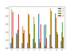
Calling a DataFrame’splot.bar() method produces a multiplebar plot:
In [21]:df2=pd.DataFrame(np.random.rand(10,4),columns=["a","b","c","d"])In [22]:df2.plot.bar();
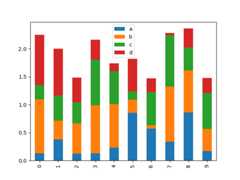
To produce a stacked bar plot, passstacked=True:
In [23]:df2.plot.bar(stacked=True);
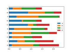
To get horizontal bar plots, use thebarh method:
In [24]:df2.plot.barh(stacked=True);
Histograms#
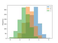
Histograms can be drawn by using theDataFrame.plot.hist() andSeries.plot.hist() methods.
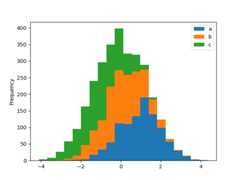
In [25]:df4=pd.DataFrame( ....:{ ....:"a":np.random.randn(1000)+1, ....:"b":np.random.randn(1000), ....:"c":np.random.randn(1000)-1, ....:}, ....:columns=["a","b","c"], ....:) ....:In [26]:plt.figure();In [27]:df4.plot.hist(alpha=0.5);
A histogram can be stacked usingstacked=True. Bin size can be changedusing thebins keyword.
In [28]:plt.figure();In [29]:df4.plot.hist(stacked=True,bins=20);
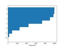
You can pass other keywords supported by matplotlibhist. For example,horizontal and cumulative histograms can be drawn byorientation='horizontal' andcumulative=True.
In [30]:plt.figure();In [31]:df4["a"].plot.hist(orientation="horizontal",cumulative=True);
See thehist method and thematplotlib hist documentation for more.
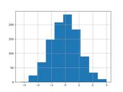
The existing interfaceDataFrame.hist to plot histogram still can be used.
In [32]:plt.figure();In [33]:df["A"].diff().hist();
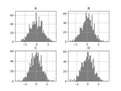
DataFrame.hist() plots the histograms of the columns on multiplesubplots:
In [34]:plt.figure();In [35]:df.diff().hist(color="k",alpha=0.5,bins=50);
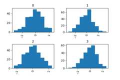
Theby keyword can be specified to plot grouped histograms:
In [36]:data=pd.Series(np.random.randn(1000))In [37]:data.hist(by=np.random.randint(0,4,1000),figsize=(6,4));
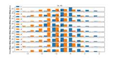
In addition, theby keyword can also be specified inDataFrame.plot.hist().
Changed in version 1.4.0.
In [38]:data=pd.DataFrame( ....:{ ....:"a":np.random.choice(["x","y","z"],1000), ....:"b":np.random.choice(["e","f","g"],1000), ....:"c":np.random.randn(1000), ....:"d":np.random.randn(1000)-1, ....:}, ....:) ....:In [39]:data.plot.hist(by=["a","b"],figsize=(10,5));
Box plots#
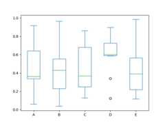
Boxplot can be drawn callingSeries.plot.box() andDataFrame.plot.box(),orDataFrame.boxplot() to visualize the distribution of values within each column.
For instance, here is a boxplot representing five trials of 10 observations ofa uniform random variable on [0,1).
In [40]:df=pd.DataFrame(np.random.rand(10,5),columns=["A","B","C","D","E"])In [41]:df.plot.box();
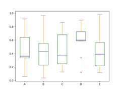
Boxplot can be colorized by passingcolor keyword. You can pass adictwhose keys areboxes,whiskers,medians andcaps.If some keys are missing in thedict, default colors are usedfor the corresponding artists. Also, boxplot hassym keyword to specify fliers style.
When you pass other type of arguments viacolor keyword, it will be directlypassed to matplotlib for all theboxes,whiskers,medians andcapscolorization.
The colors are applied to every boxes to be drawn. If you wantmore complicated colorization, you can get each drawn artists by passingreturn_type.
In [42]:color={ ....:"boxes":"DarkGreen", ....:"whiskers":"DarkOrange", ....:"medians":"DarkBlue", ....:"caps":"Gray", ....:} ....:In [43]:df.plot.box(color=color,sym="r+");
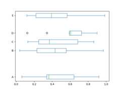
Also, you can pass other keywords supported by matplotlibboxplot.For example, horizontal and custom-positioned boxplot can be drawn byvert=False andpositions keywords.
In [44]:df.plot.box(vert=False,positions=[1,4,5,6,8]);
See theboxplot method and thematplotlib boxplot documentation for more.
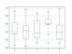
The existing interfaceDataFrame.boxplot to plot boxplot still can be used.
In [45]:df=pd.DataFrame(np.random.rand(10,5))In [46]:plt.figure();In [47]:bp=df.boxplot()
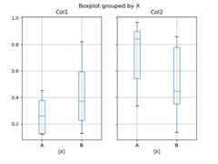
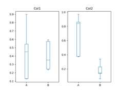
You can create a stratified boxplot using theby keyword argument to creategroupings. For instance,
In [48]:df=pd.DataFrame(np.random.rand(10,2),columns=["Col1","Col2"])In [49]:df["X"]=pd.Series(["A","A","A","A","A","B","B","B","B","B"])In [50]:plt.figure();In [51]:bp=df.boxplot(by="X")
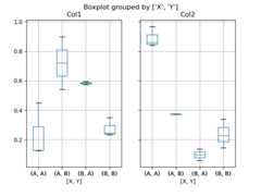
You can also pass a subset of columns to plot, as well as group by multiplecolumns:
In [52]:df=pd.DataFrame(np.random.rand(10,3),columns=["Col1","Col2","Col3"])In [53]:df["X"]=pd.Series(["A","A","A","A","A","B","B","B","B","B"])In [54]:df["Y"]=pd.Series(["A","B","A","B","A","B","A","B","A","B"])In [55]:plt.figure();In [56]:bp=df.boxplot(column=["Col1","Col2"],by=["X","Y"])
You could also create groupings withDataFrame.plot.box(), for instance:
Changed in version 1.4.0.
In [57]:df=pd.DataFrame(np.random.rand(10,3),columns=["Col1","Col2","Col3"])In [58]:df["X"]=pd.Series(["A","A","A","A","A","B","B","B","B","B"])In [59]:plt.figure();In [60]:bp=df.plot.box(column=["Col1","Col2"],by="X")
Inboxplot, the return type can be controlled by thereturn_type, keyword. The valid choices are{"axes","dict","both",None}.Faceting, created byDataFrame.boxplot with thebykeyword, will affect the output type as well:
| Faceted | Output type |
|---|---|---|
| No | axes |
| Yes | 2-D ndarray of axes |
| No | axes |
| Yes | Series of axes |
| No | dict of artists |
| Yes | Series of dicts of artists |
| No | namedtuple |
| Yes | Series of namedtuples |
Groupby.boxplot always returns aSeries ofreturn_type.
In [61]:np.random.seed(1234)In [62]:df_box=pd.DataFrame(np.random.randn(50,2))In [63]:df_box["g"]=np.random.choice(["A","B"],size=50)In [64]:df_box.loc[df_box["g"]=="B",1]+=3In [65]:bp=df_box.boxplot(by="g")
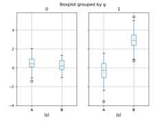
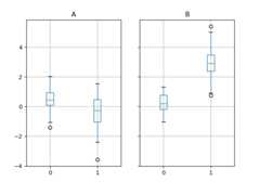
The subplots above are split by the numeric columns first, then the value oftheg column. Below the subplots are first split by the value ofg,then by the numeric columns.
In [66]:bp=df_box.groupby("g").boxplot()
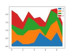
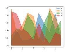
Area plot#
You can create area plots withSeries.plot.area() andDataFrame.plot.area().Area plots are stacked by default. To produce stacked area plot, each column must be either all positive or all negative values.
When input data containsNaN, it will be automatically filled by 0. If you want to drop or fill by different values, usedataframe.dropna() ordataframe.fillna() before callingplot.
In [67]:df=pd.DataFrame(np.random.rand(10,4),columns=["a","b","c","d"])In [68]:df.plot.area();
To produce an unstacked plot, passstacked=False. Alpha value is set to 0.5 unless otherwise specified:
In [69]:df.plot.area(stacked=False);
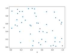
Scatter plot#
Scatter plot can be drawn by using theDataFrame.plot.scatter() method.Scatter plot requires numeric columns for the x and y axes.These can be specified by thex andy keywords.
In [70]:df=pd.DataFrame(np.random.rand(50,4),columns=["a","b","c","d"])In [71]:df["species"]=pd.Categorical( ....:["setosa"]*20+["versicolor"]*20+["virginica"]*10 ....:) ....:In [72]:df.plot.scatter(x="a",y="b");
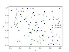
To plot multiple column groups in a single axes, repeatplot method specifying targetax.It is recommended to specifycolor andlabel keywords to distinguish each groups.
In [73]:ax=df.plot.scatter(x="a",y="b",color="DarkBlue",label="Group 1")In [74]:df.plot.scatter(x="c",y="d",color="DarkGreen",label="Group 2",ax=ax);
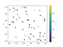
The keywordc may be given as the name of a column to provide colors foreach point:
In [75]:df.plot.scatter(x="a",y="b",c="c",s=50);
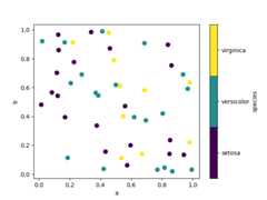
If a categorical column is passed toc, then a discrete colorbar will be produced:
Added in version 1.3.0.
In [76]:df.plot.scatter(x="a",y="b",c="species",cmap="viridis",s=50);
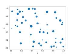
You can pass other keywords supported by matplotlibscatter. The example below shows abubble chart using a column of theDataFrame as the bubble size.
In [77]:df.plot.scatter(x="a",y="b",s=df["c"]*200);
See thescatter method and thematplotlib scatter documentation for more.
Hexagonal bin plot#
You can create hexagonal bin plots withDataFrame.plot.hexbin().Hexbin plots can be a useful alternative to scatter plots if your data aretoo dense to plot each point individually.
In [78]:df=pd.DataFrame(np.random.randn(1000,2),columns=["a","b"])In [79]:df["b"]=df["b"]+np.arange(1000)In [80]:df.plot.hexbin(x="a",y="b",gridsize=25);
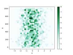
A useful keyword argument isgridsize; it controls the number of hexagonsin the x-direction, and defaults to 100. A largergridsize means more, smallerbins.
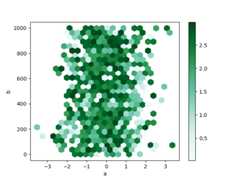
By default, a histogram of the counts around each(x,y) point is computed.You can specify alternative aggregations by passing values to theC andreduce_C_function arguments.C specifies the value at each(x,y) pointandreduce_C_function is a function of one argument that reduces all thevalues in a bin to a single number (e.g.mean,max,sum,std). In thisexample the positions are given by columnsa andb, while the value isgiven by columnz. The bins are aggregated with NumPy’smax function.
In [81]:df=pd.DataFrame(np.random.randn(1000,2),columns=["a","b"])In [82]:df["b"]=df["b"]+np.arange(1000)In [83]:df["z"]=np.random.uniform(0,3,1000)In [84]:df.plot.hexbin(x="a",y="b",C="z",reduce_C_function=np.max,gridsize=25);
See thehexbin method and thematplotlib hexbin documentation for more.
Pie plot#
You can create a pie plot withDataFrame.plot.pie() orSeries.plot.pie().If your data includes anyNaN, they will be automatically filled with 0.AValueError will be raised if there are any negative values in your data.
In [85]:series=pd.Series(3*np.random.rand(4),index=["a","b","c","d"],name="series")In [86]:series.plot.pie(figsize=(6,6));
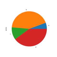
For pie plots it’s best to use square figures, i.e. a figure aspect ratio 1.You can create the figure with equal width and height, or force the aspect ratioto be equal after plotting by callingax.set_aspect('equal') on the returnedaxes object.
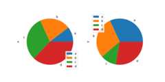
Note that pie plot withDataFrame requires that you either specify atarget column by they argument orsubplots=True. Wheny isspecified, pie plot of selected column will be drawn. Ifsubplots=True isspecified, pie plots for each column are drawn as subplots. A legend will bedrawn in each pie plots by default; specifylegend=False to hide it.
In [87]:df=pd.DataFrame( ....:3*np.random.rand(4,2),index=["a","b","c","d"],columns=["x","y"] ....:) ....:In [88]:df.plot.pie(subplots=True,figsize=(8,4));
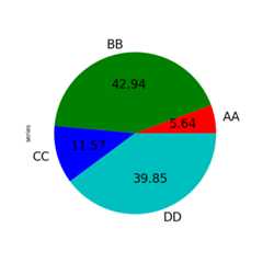
You can use thelabels andcolors keywords to specify the labels and colors of each wedge.
Warning
Most pandas plots use thelabel andcolor arguments (note the lack of “s” on those).To be consistent withmatplotlib.pyplot.pie() you must uselabels andcolors.
If you want to hide wedge labels, specifylabels=None.Iffontsize is specified, the value will be applied to wedge labels.Also, other keywords supported bymatplotlib.pyplot.pie() can be used.
In [89]:series.plot.pie( ....:labels=["AA","BB","CC","DD"], ....:colors=["r","g","b","c"], ....:autopct="%.2f", ....:fontsize=20, ....:figsize=(6,6), ....:); ....:
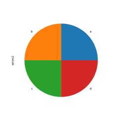
If you pass values whose sum total is less than 1.0 they will be rescaled so that they sum to 1.
In [90]:series=pd.Series([0.1]*4,index=["a","b","c","d"],name="series2")In [91]:series.plot.pie(figsize=(6,6));
See thematplotlib pie documentation for more.
Plotting with missing data#
pandas tries to be pragmatic about plottingDataFrames orSeriesthat contain missing data. Missing values are dropped, left out, or filleddepending on the plot type.
Plot Type | NaN Handling |
|---|---|
Line | Leave gaps at NaNs |
Line (stacked) | Fill 0’s |
Bar | Fill 0’s |
Scatter | Drop NaNs |
Histogram | Drop NaNs (column-wise) |
Box | Drop NaNs (column-wise) |
Area | Fill 0’s |
KDE | Drop NaNs (column-wise) |
Hexbin | Drop NaNs |
Pie | Fill 0’s |
If any of these defaults are not what you want, or if you want to beexplicit about how missing values are handled, consider usingfillna() ordropna()before plotting.
Plotting tools#
These functions can be imported frompandas.plottingand take aSeries orDataFrame as an argument.
Scatter matrix plot#
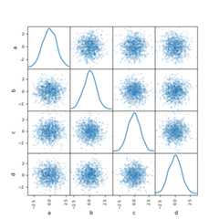
You can create a scatter plot matrix using thescatter_matrix method inpandas.plotting:
In [92]:frompandas.plottingimportscatter_matrixIn [93]:df=pd.DataFrame(np.random.randn(1000,4),columns=["a","b","c","d"])In [94]:scatter_matrix(df,alpha=0.2,figsize=(6,6),diagonal="kde");
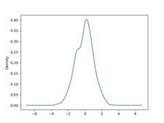
Density plot#
You can create density plots using theSeries.plot.kde() andDataFrame.plot.kde() methods.
In [95]:ser=pd.Series(np.random.randn(1000))In [96]:ser.plot.kde();
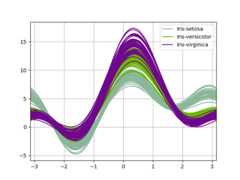
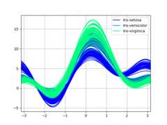
Andrews curves#
Andrews curves allow one to plot multivariate data as a large numberof curves that are created using the attributes of samples as coefficientsfor Fourier series, see theWikipedia entryfor more information. By coloring these curves differently for each classit is possible to visualize data clustering. Curves belonging to samplesof the same class will usually be closer together and form larger structures.
Note: The “Iris” dataset is availablehere.
In [97]:frompandas.plottingimportandrews_curvesIn [98]:data=pd.read_csv("data/iris.data")In [99]:plt.figure();In [100]:andrews_curves(data,"Name");
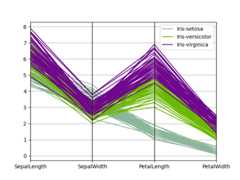
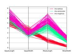
Parallel coordinates#
Parallel coordinates is a plotting technique for plotting multivariate data,see theWikipedia entryfor an introduction.Parallel coordinates allows one to see clusters in data and to estimate other statistics visually.Using parallel coordinates points are represented as connected line segments.Each vertical line represents one attribute. One set of connected line segmentsrepresents one data point. Points that tend to cluster will appear closer together.
In [101]:frompandas.plottingimportparallel_coordinatesIn [102]:data=pd.read_csv("data/iris.data")In [103]:plt.figure();In [104]:parallel_coordinates(data,"Name");
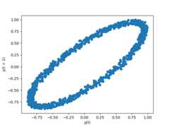
Lag plot#
Lag plots are used to check if a data set or time series is random. Randomdata should not exhibit any structure in the lag plot. Non-random structureimplies that the underlying data are not random. Thelag argument maybe passed, and whenlag=1 the plot is essentiallydata[:-1] vs.data[1:].
In [105]:frompandas.plottingimportlag_plotIn [106]:plt.figure();In [107]:spacing=np.linspace(-99*np.pi,99*np.pi,num=1000)In [108]:data=pd.Series(0.1*np.random.rand(1000)+0.9*np.sin(spacing))In [109]:lag_plot(data);
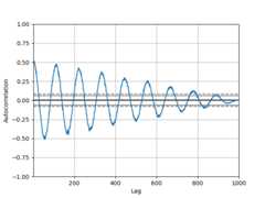
Autocorrelation plot#
Autocorrelation plots are often used for checking randomness in time series.This is done by computing autocorrelations for data values at varying time lags.If time series is random, such autocorrelations should be near zero for any andall time-lag separations. If time series is non-random then one or more of theautocorrelations will be significantly non-zero. The horizontal lines displayedin the plot correspond to 95% and 99% confidence bands. The dashed line is 99%confidence band. See theWikipedia entry for more aboutautocorrelation plots.
In [110]:frompandas.plottingimportautocorrelation_plotIn [111]:plt.figure();In [112]:spacing=np.linspace(-9*np.pi,9*np.pi,num=1000)In [113]:data=pd.Series(0.7*np.random.rand(1000)+0.3*np.sin(spacing))In [114]:autocorrelation_plot(data);
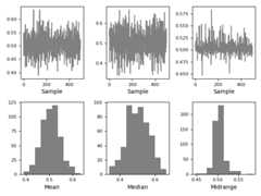
Bootstrap plot#
Bootstrap plots are used to visually assess the uncertainty of a statistic, suchas mean, median, midrange, etc. A random subset of a specified size is selectedfrom a data set, the statistic in question is computed for this subset and theprocess is repeated a specified number of times. Resulting plots and histogramsare what constitutes the bootstrap plot.
In [115]:frompandas.plottingimportbootstrap_plotIn [116]:data=pd.Series(np.random.rand(1000))In [117]:bootstrap_plot(data,size=50,samples=500,color="grey");
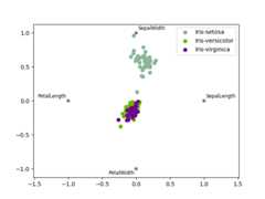
RadViz#
RadViz is a way of visualizing multi-variate data. It is based on a simplespring tension minimization algorithm. Basically you set up a bunch of points ina plane. In our case they are equally spaced on a unit circle. Each pointrepresents a single attribute. You then pretend that each sample in the data setis attached to each of these points by a spring, the stiffness of which isproportional to the numerical value of that attribute (they are normalized tounit interval). The point in the plane, where our sample settles to (where theforces acting on our sample are at an equilibrium) is where a dot representingour sample will be drawn. Depending on which class that sample belongs it willbe colored differently.See the R packageRadvizfor more information.
Note: The “Iris” dataset is availablehere.
In [118]:frompandas.plottingimportradvizIn [119]:data=pd.read_csv("data/iris.data")In [120]:plt.figure();In [121]:radviz(data,"Name");
Plot formatting#
Setting the plot style#
From version 1.5 and up, matplotlib offers a range of pre-configured plotting styles. Setting thestyle can be used to easily give plots the general look that you want.Setting the style is as easy as callingmatplotlib.style.use(my_plot_style) beforecreating your plot. For example you could writematplotlib.style.use('ggplot') for ggplot-styleplots.
You can see the various available style names atmatplotlib.style.available and it’s veryeasy to try them out.
General plot style arguments#
Most plotting methods have a set of keyword arguments that control thelayout and formatting of the returned plot:
In [122]:plt.figure();In [123]:ts.plot(style="k--",label="Series");
For each kind of plot (e.g.line,bar,scatter) any additional argumentskeywords are passed along to the corresponding matplotlib function(ax.plot(),ax.bar(),ax.scatter()). These can be usedto control additional styling, beyond what pandas provides.
Controlling the legend#
You may set thelegend argument toFalse to hide the legend, which isshown by default.
In [124]:df=pd.DataFrame(np.random.randn(1000,4),index=ts.index,columns=list("ABCD"))In [125]:df=df.cumsum()In [126]:df.plot(legend=False);
Controlling the labels#
You may set thexlabel andylabel arguments to give the plot custom labelsfor x and y axis. By default, pandas will pick up index name as xlabel, while leavingit empty for ylabel.
In [127]:df.plot();In [128]:df.plot(xlabel="new x",ylabel="new y");
Scales#
You may passlogy to get a log-scale Y axis.
In [129]:ts=pd.Series(np.random.randn(1000),index=pd.date_range("1/1/2000",periods=1000))In [130]:ts=np.exp(ts.cumsum())In [131]:ts.plot(logy=True);
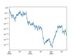
See also thelogx andloglog keyword arguments.
Plotting on a secondary y-axis#
To plot data on a secondary y-axis, use thesecondary_y keyword:
In [132]:df["A"].plot();In [133]:df["B"].plot(secondary_y=True,style="g");
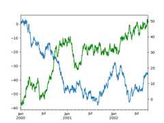
To plot some columns in aDataFrame, give the column names to thesecondary_ykeyword:
In [134]:plt.figure();In [135]:ax=df.plot(secondary_y=["A","B"])In [136]:ax.set_ylabel("CD scale");In [137]:ax.right_ax.set_ylabel("AB scale");
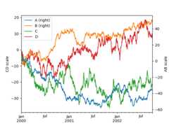
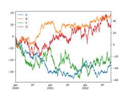
Note that the columns plotted on the secondary y-axis is automatically markedwith “(right)” in the legend. To turn off the automatic marking, use themark_right=False keyword:
In [138]:plt.figure();In [139]:df.plot(secondary_y=["A","B"],mark_right=False);
Custom formatters for timeseries plots#
pandas provides custom formatters for timeseries plots. These change theformatting of the axis labels for dates and times. By default,the custom formatters are applied only to plots created by pandas withDataFrame.plot() orSeries.plot(). To have them apply to allplots, including those made by matplotlib, set the optionpd.options.plotting.matplotlib.register_converters=True or usepandas.plotting.register_matplotlib_converters().
Suppressing tick resolution adjustment#
pandas includes automatic tick resolution adjustment for regular frequencytime-series data. For limited cases where pandas cannot infer the frequencyinformation (e.g., in an externally createdtwinx), you can choose tosuppress this behavior for alignment purposes.
Here is the default behavior, notice how the x-axis tick labeling is performed:
In [140]:plt.figure();In [141]:df["A"].plot();
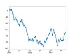
Using thex_compat parameter, you can suppress this behavior:
In [142]:plt.figure();In [143]:df["A"].plot(x_compat=True);
If you have more than one plot that needs to be suppressed, theuse methodinpandas.plotting.plot_params can be used in awith statement:
In [144]:plt.figure();In [145]:withpd.plotting.plot_params.use("x_compat",True): .....:df["A"].plot(color="r") .....:df["B"].plot(color="g") .....:df["C"].plot(color="b") .....:
Automatic date tick adjustment#
TimedeltaIndex now uses the native matplotlibtick locator methods, it is useful to call the automaticdate tick adjustment from matplotlib for figures whose ticklabels overlap.
See theautofmt_xdate method and thematplotlib documentation for more.
Subplots#
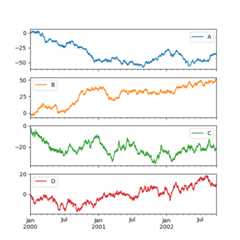
EachSeries in aDataFrame can be plotted on a different axiswith thesubplots keyword:
In [146]:df.plot(subplots=True,figsize=(6,6));
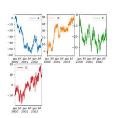
Using layout and targeting multiple axes#
The layout of subplots can be specified by thelayout keyword. It can accept(rows,columns). Thelayout keyword can be used inhist andboxplot also. If the input is invalid, aValueError will be raised.
The number of axes which can be contained by rows x columns specified bylayout must belarger than the number of required subplots. If layout can contain more axes than required,blank axes are not drawn. Similar to a NumPy array’sreshape method, youcan use-1 for one dimension to automatically calculate the number of rowsor columns needed, given the other.
In [147]:df.plot(subplots=True,layout=(2,3),figsize=(6,6),sharex=False);
The above example is identical to using:
In [148]:df.plot(subplots=True,layout=(2,-1),figsize=(6,6),sharex=False);
The required number of columns (3) is inferred from the number of series to plotand the given number of rows (2).
You can pass multiple axes created beforehand as list-like viaax keyword.This allows more complicated layouts.The passed axes must be the same number as the subplots being drawn.
When multiple axes are passed via theax keyword,layout,sharex andsharey keywordsdon’t affect to the output. You should explicitly passsharex=False andsharey=False,otherwise you will see a warning.
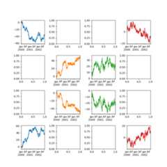
In [149]:fig,axes=plt.subplots(4,4,figsize=(9,9))In [150]:plt.subplots_adjust(wspace=0.5,hspace=0.5)In [151]:target1=[axes[0][0],axes[1][1],axes[2][2],axes[3][3]]In [152]:target2=[axes[3][0],axes[2][1],axes[1][2],axes[0][3]]In [153]:df.plot(subplots=True,ax=target1,legend=False,sharex=False,sharey=False);In [154]:(-df).plot(subplots=True,ax=target2,legend=False,sharex=False,sharey=False);
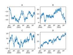
Another option is passing anax argument toSeries.plot() to plot on a particular axis:
In [155]:np.random.seed(123456)In [156]:ts=pd.Series(np.random.randn(1000),index=pd.date_range("1/1/2000",periods=1000))In [157]:ts=ts.cumsum()In [158]:df=pd.DataFrame(np.random.randn(1000,4),index=ts.index,columns=list("ABCD"))In [159]:df=df.cumsum()
In [160]:fig,axes=plt.subplots(nrows=2,ncols=2)In [161]:plt.subplots_adjust(wspace=0.2,hspace=0.5)In [162]:df["A"].plot(ax=axes[0,0]);In [163]:axes[0,0].set_title("A");In [164]:df["B"].plot(ax=axes[0,1]);In [165]:axes[0,1].set_title("B");In [166]:df["C"].plot(ax=axes[1,0]);In [167]:axes[1,0].set_title("C");In [168]:df["D"].plot(ax=axes[1,1]);In [169]:axes[1,1].set_title("D");
Plotting with error bars#
Plotting with error bars is supported inDataFrame.plot() andSeries.plot().
Horizontal and vertical error bars can be supplied to thexerr andyerr keyword arguments toplot(). The error values can be specified using a variety of formats:
As a
DataFrameordictof errors with column names matching thecolumnsattribute of the plottingDataFrameor matching thenameattribute of theSeries.As a
strindicating which of the columns of plottingDataFramecontain the error values.As raw values (
list,tuple, ornp.ndarray). Must be the same length as the plottingDataFrame/Series.
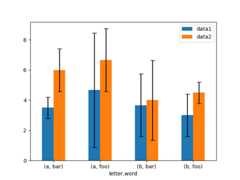
Here is an example of one way to easily plot group means with standard deviations from the raw data.
# Generate the dataIn [170]:ix3=pd.MultiIndex.from_arrays( .....:[ .....:["a","a","a","a","a","b","b","b","b","b"], .....:["foo","foo","foo","bar","bar","foo","foo","bar","bar","bar"], .....:], .....:names=["letter","word"], .....:) .....:In [171]:df3=pd.DataFrame( .....:{ .....:"data1":[9,3,2,4,3,2,4,6,3,2], .....:"data2":[9,6,5,7,5,4,5,6,5,1], .....:}, .....:index=ix3, .....:) .....:# Group by index labels and take the means and standard deviations# for each groupIn [172]:gp3=df3.groupby(level=("letter","word"))In [173]:means=gp3.mean()In [174]:errors=gp3.std()In [175]:meansOut[175]: data1 data2letter worda bar 3.500000 6.000000 foo 4.666667 6.666667b bar 3.666667 4.000000 foo 3.000000 4.500000In [176]:errorsOut[176]: data1 data2letter worda bar 0.707107 1.414214 foo 3.785939 2.081666b bar 2.081666 2.645751 foo 1.414214 0.707107# PlotIn [177]:fig,ax=plt.subplots()In [178]:means.plot.bar(yerr=errors,ax=ax,capsize=4,rot=0);
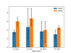
Asymmetrical error bars are also supported, however raw error values must be provided in this case. For aN lengthSeries, a2xN array should be provided indicating lower and upper (or left and right) errors. For aMxNDataFrame, asymmetrical errors should be in aMx2xN array.
Here is an example of one way to plot the min/max range using asymmetrical error bars.
In [179]:mins=gp3.min()In [180]:maxs=gp3.max()# errors should be positive, and defined in the order of lower, upperIn [181]:errors=[[means[c]-mins[c],maxs[c]-means[c]]forcindf3.columns]# PlotIn [182]:fig,ax=plt.subplots()In [183]:means.plot.bar(yerr=errors,ax=ax,capsize=4,rot=0);
Plotting tables#
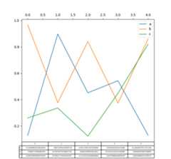
Plotting with matplotlib table is now supported inDataFrame.plot() andSeries.plot() with atable keyword. Thetable keyword can acceptbool,DataFrame orSeries. The simple way to draw a table is to specifytable=True. Data will be transposed to meet matplotlib’s default layout.
In [184]:np.random.seed(123456)In [185]:fig,ax=plt.subplots(1,1,figsize=(7,6.5))In [186]:df=pd.DataFrame(np.random.rand(5,3),columns=["a","b","c"])In [187]:ax.xaxis.tick_top()# Display x-axis ticks on top.In [188]:df.plot(table=True,ax=ax);
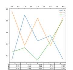
Also, you can pass a differentDataFrame orSeries to thetable keyword. The data will be drawn as displayed in print method(not transposed automatically). If required, it should be transposed manuallyas seen in the example below.
In [189]:fig,ax=plt.subplots(1,1,figsize=(7,6.75))In [190]:ax.xaxis.tick_top()# Display x-axis ticks on top.In [191]:df.plot(table=np.round(df.T,2),ax=ax);
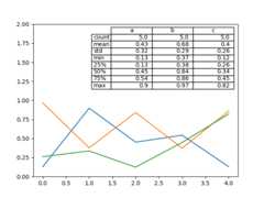
There also exists a helper functionpandas.plotting.table, which creates atable fromDataFrame orSeries, and adds it to anmatplotlib.Axes instance. This function can accept keywords which thematplotlibtable has.
In [192]:frompandas.plottingimporttableIn [193]:fig,ax=plt.subplots(1,1)In [194]:table(ax,np.round(df.describe(),2),loc="upper right",colWidths=[0.2,0.2,0.2]);In [195]:df.plot(ax=ax,ylim=(0,2),legend=None);
Note: You can get table instances on the axes usingaxes.tables property for further decorations. See thematplotlib table documentation for more.
Colormaps#
A potential issue when plotting a large number of columns is that it can bedifficult to distinguish some series due to repetition in the default colors. Toremedy this,DataFrame plotting supports the use of thecolormap argument,which accepts either a Matplotlibcolormapor a string that is a name of a colormap registered with Matplotlib. Avisualization of the default matplotlib colormaps is availablehere.
As matplotlib does not directly support colormaps for line-based plots, thecolors are selected based on an even spacing determined by the number of columnsin theDataFrame. There is no consideration made for background color, so somecolormaps will produce lines that are not easily visible.
To use the cubehelix colormap, we can passcolormap='cubehelix'.
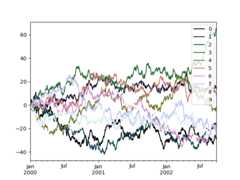
In [196]:np.random.seed(123456)In [197]:df=pd.DataFrame(np.random.randn(1000,10),index=ts.index)In [198]:df=df.cumsum()In [199]:plt.figure();In [200]:df.plot(colormap="cubehelix");
Alternatively, we can pass the colormap itself:
In [201]:frommatplotlibimportcmIn [202]:plt.figure();In [203]:df.plot(colormap=cm.cubehelix);

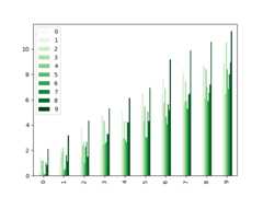
Colormaps can also be used other plot types, like bar charts:
In [204]:np.random.seed(123456)In [205]:dd=pd.DataFrame(np.random.randn(10,10)).map(abs)In [206]:dd=dd.cumsum()In [207]:plt.figure();In [208]:dd.plot.bar(colormap="Greens");
Parallel coordinates charts:
In [209]:plt.figure();In [210]:parallel_coordinates(data,"Name",colormap="gist_rainbow");
Andrews curves charts:
In [211]:plt.figure();In [212]:andrews_curves(data,"Name",colormap="winter");
Plotting directly with Matplotlib#
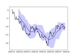
In some situations it may still be preferable or necessary to prepare plotsdirectly with matplotlib, for instance when a certain type of plot orcustomization is not (yet) supported by pandas.Series andDataFrameobjects behave like arrays and can therefore be passed directly tomatplotlib functions without explicit casts.
pandas also automatically registers formatters and locators that recognize dateindices, thereby extending date and time support to practically all plot typesavailable in matplotlib. Although this formatting does not provide the samelevel of refinement you would get when plotting via pandas, it can be fasterwhen plotting a large number of points.
In [213]:np.random.seed(123456)In [214]:price=pd.Series( .....:np.random.randn(150).cumsum(), .....:index=pd.date_range("2000-1-1",periods=150,freq="B"), .....:) .....:In [215]:ma=price.rolling(20).mean()In [216]:mstd=price.rolling(20).std()In [217]:plt.figure();In [218]:plt.plot(price.index,price,"k");In [219]:plt.plot(ma.index,ma,"b");In [220]:plt.fill_between(mstd.index,ma-2*mstd,ma+2*mstd,color="b",alpha=0.2);
Plotting backends#
pandas can be extended with third-party plotting backends. Themain idea is letting users select a plotting backend different than the providedone based on Matplotlib.
This can be done by passing ‘backend.module’ as the argumentbackend inplotfunction. For example:
>>>Series([1,2,3]).plot(backend="backend.module")
Alternatively, you can also set this option globally, do you don’t need to specifythe keyword in eachplot call. For example:
>>>pd.set_option("plotting.backend","backend.module")>>>pd.Series([1,2,3]).plot()
Or:
>>>pd.options.plotting.backend="backend.module">>>pd.Series([1,2,3]).plot()
This would be more or less equivalent to:
>>>importbackend.module>>>backend.module.plot(pd.Series([1,2,3]))
The backend module can then use other visualization tools (Bokeh, Altair, hvplot,…)to generate the plots. Some libraries implementing a backend for pandas are listedonthe ecosystem page.
Developers guide can be found athttps://pandas.pydata.org/docs/dev/development/extending.html#plotting-backends