Reshaping and pivot tables#
pandas provides methods for manipulating aSeries andDataFrame to alter therepresentation of the data for further data processing or data summarization.
pivot()andpivot_table(): Group unique values within one or more discrete categories.stack()andunstack(): Pivot a column or row level to the opposite axis respectively.melt()andwide_to_long(): Unpivot a wideDataFrameto a long format.get_dummies()andfrom_dummies(): Conversions with indicator variables.explode(): Convert a column of list-like values to individual rows.crosstab(): Calculate a cross-tabulation of multiple 1 dimensional factor arrays.cut(): Transform continuous variables to discrete, categorical valuesfactorize(): Encode 1 dimensional variables into integer labels.
pivot() andpivot_table()#
pivot()#
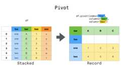
Data is often stored in so-called “stacked” or “record” format. In a “record” or “wide” format,typically there is one row for each subject. In the “stacked” or “long” format there aremultiple rows for each subject where applicable.
In [1]:data={ ...:"value":range(12), ...:"variable":["A"]*3+["B"]*3+["C"]*3+["D"]*3, ...:"date":pd.to_datetime(["2020-01-03","2020-01-04","2020-01-05"]*4) ...:} ...:In [2]:df=pd.DataFrame(data)
To perform time series operations with each unique variable, a betterrepresentation would be where thecolumns are the unique variables and anindex of dates identifies individual observations. To reshape the data intothis form, we use theDataFrame.pivot() method (also implemented as atop level functionpivot()):
In [3]:pivoted=df.pivot(index="date",columns="variable",values="value")In [4]:pivotedOut[4]:variable A B C Ddate2020-01-03 0 3 6 92020-01-04 1 4 7 102020-01-05 2 5 8 11
If thevalues argument is omitted, and the inputDataFrame has more thanone column of values which are not used as column or index inputs topivot(),then the resulting “pivoted”DataFrame will havehierarchical columns whose topmost level indicates the respective valuecolumn:
In [5]:df["value2"]=df["value"]*2In [6]:pivoted=df.pivot(index="date",columns="variable")In [7]:pivotedOut[7]: value value2variable A B C D A B C Ddate2020-01-03 0 3 6 9 0 6 12 182020-01-04 1 4 7 10 2 8 14 202020-01-05 2 5 8 11 4 10 16 22
You can then select subsets from the pivotedDataFrame:
In [8]:pivoted["value2"]Out[8]:variable A B C Ddate2020-01-03 0 6 12 182020-01-04 2 8 14 202020-01-05 4 10 16 22
Note that this returns a view on the underlying data in the case where the dataare homogeneously-typed.
Note
pivot() can only handle unique rows specified byindex andcolumns.If you data contains duplicates, usepivot_table().
pivot_table()#
Whilepivot() provides general purpose pivoting with variousdata types, pandas also providespivot_table() orpivot_table()for pivoting with aggregation of numeric data.
The functionpivot_table() can be used to create spreadsheet-stylepivot tables. See thecookbook for some advancedstrategies.
In [9]:importdatetimeIn [10]:df=pd.DataFrame( ....:{ ....:"A":["one","one","two","three"]*6, ....:"B":["A","B","C"]*8, ....:"C":["foo","foo","foo","bar","bar","bar"]*4, ....:"D":np.random.randn(24), ....:"E":np.random.randn(24), ....:"F":[datetime.datetime(2013,i,1)foriinrange(1,13)] ....:+[datetime.datetime(2013,i,15)foriinrange(1,13)], ....:} ....:) ....:In [11]:dfOut[11]: A B C D E F0 one A foo 0.469112 0.404705 2013-01-011 one B foo -0.282863 0.577046 2013-02-012 two C foo -1.509059 -1.715002 2013-03-013 three A bar -1.135632 -1.039268 2013-04-014 one B bar 1.212112 -0.370647 2013-05-01.. ... .. ... ... ... ...19 three B foo -1.087401 -0.472035 2013-08-1520 one C foo -0.673690 -0.013960 2013-09-1521 one A bar 0.113648 -0.362543 2013-10-1522 two B bar -1.478427 -0.006154 2013-11-1523 three C bar 0.524988 -0.923061 2013-12-15[24 rows x 6 columns]In [12]:pd.pivot_table(df,values="D",index=["A","B"],columns=["C"])Out[12]:C bar fooA Bone A -0.995460 0.595334 B 0.393570 -0.494817 C 0.196903 -0.767769three A -0.431886 NaN B NaN -1.065818 C 0.798396 NaNtwo A NaN 0.197720 B -0.986678 NaN C NaN -1.274317In [13]:pd.pivot_table( ....:df,values=["D","E"], ....:index=["B"], ....:columns=["A","C"], ....:aggfunc="sum", ....:) ....:Out[13]: D ... EA one three ... three twoC bar foo bar ... foo bar fooB ...A -1.990921 1.190667 -0.863772 ... NaN NaN -1.067650B 0.787140 -0.989634 NaN ... 0.372851 1.63741 NaNC 0.393806 -1.535539 1.596791 ... NaN NaN -3.491906[3 rows x 12 columns]In [14]:pd.pivot_table( ....:df,values="E", ....:index=["B","C"], ....:columns=["A"], ....:aggfunc=["sum","mean"], ....:) ....:Out[14]: sum meanA one three two one three twoB CA bar -0.471593 -2.008182 NaN -0.235796 -1.004091 NaN foo 0.761726 NaN -1.067650 0.380863 NaN -0.533825B bar -1.665170 NaN 1.637410 -0.832585 NaN 0.818705 foo -0.097554 0.372851 NaN -0.048777 0.186425 NaNC bar -0.744154 -2.392449 NaN -0.372077 -1.196224 NaN foo 1.061810 NaN -3.491906 0.530905 NaN -1.745953
The result is aDataFrame potentially having aMultiIndex on theindex or column. If thevalues column name is not given, the pivot tablewill include all of the data in an additional level of hierarchy in the columns:
In [15]:pd.pivot_table(df[["A","B","C","D","E"]],index=["A","B"],columns=["C"])Out[15]: D EC bar foo bar fooA Bone A -0.995460 0.595334 -0.235796 0.380863 B 0.393570 -0.494817 -0.832585 -0.048777 C 0.196903 -0.767769 -0.372077 0.530905three A -0.431886 NaN -1.004091 NaN B NaN -1.065818 NaN 0.186425 C 0.798396 NaN -1.196224 NaNtwo A NaN 0.197720 NaN -0.533825 B -0.986678 NaN 0.818705 NaN C NaN -1.274317 NaN -1.745953
Also, you can useGrouper forindex andcolumns keywords. For detail ofGrouper, seeGrouping with a Grouper specification.
In [16]:pd.pivot_table(df,values="D",index=pd.Grouper(freq="ME",key="F"),columns="C")Out[16]:C bar fooF2013-01-31 NaN 0.5953342013-02-28 NaN -0.4948172013-03-31 NaN -1.2743172013-04-30 -0.431886 NaN2013-05-31 0.393570 NaN2013-06-30 0.196903 NaN2013-07-31 NaN 0.1977202013-08-31 NaN -1.0658182013-09-30 NaN -0.7677692013-10-31 -0.995460 NaN2013-11-30 -0.986678 NaN2013-12-31 0.798396 NaN
Adding margins#
Passingmargins=True topivot_table() will add a row and column with anAll label with partial group aggregates across the categories on therows and columns:
In [17]:table=df.pivot_table( ....:index=["A","B"], ....:columns="C", ....:values=["D","E"], ....:margins=True, ....:aggfunc="std" ....:) ....:In [18]:tableOut[18]: D EC bar foo All bar foo AllA Bone A 1.568517 0.178504 1.293926 0.179247 0.033718 0.371275 B 1.157593 0.299748 0.860059 0.653280 0.885047 0.779837 C 0.523425 0.133049 0.638297 1.111310 0.770555 0.938819three A 0.995247 NaN 0.995247 0.049748 NaN 0.049748 B NaN 0.030522 0.030522 NaN 0.931203 0.931203 C 0.386657 NaN 0.386657 0.386312 NaN 0.386312two A NaN 0.111032 0.111032 NaN 1.146201 1.146201 B 0.695438 NaN 0.695438 1.166526 NaN 1.166526 C NaN 0.331975 0.331975 NaN 0.043771 0.043771All 1.014073 0.713941 0.871016 0.881376 0.984017 0.923568
Additionally, you can callDataFrame.stack() to display a pivoted DataFrameas having a multi-level index:
In [19]:table.stack(future_stack=True)Out[19]: D EA B Cone A bar 1.568517 0.179247 foo 0.178504 0.033718 All 1.293926 0.371275 B bar 1.157593 0.653280 foo 0.299748 0.885047... ... ...two C foo 0.331975 0.043771 All 0.331975 0.043771All bar 1.014073 0.881376 foo 0.713941 0.984017 All 0.871016 0.923568[30 rows x 2 columns]
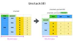
stack() andunstack()#
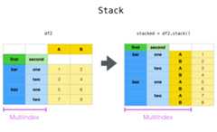
Closely related to thepivot() method are the relatedstack() andunstack() methods available onSeries andDataFrame. These methods are designed to work together withMultiIndex objects (see the section onhierarchical indexing).
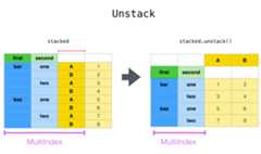
stack(): “pivot” a level of the (possibly hierarchical) column labels,returning aDataFramewith an index with a new inner-most level of rowlabels.unstack(): (inverse operation ofstack()) “pivot” a level of the(possibly hierarchical) row index to the column axis, producing a reshapedDataFramewith a new inner-most level of column labels.
In [20]:tuples=[ ....:["bar","bar","baz","baz","foo","foo","qux","qux"], ....:["one","two","one","two","one","two","one","two"], ....:] ....:In [21]:index=pd.MultiIndex.from_arrays(tuples,names=["first","second"])In [22]:df=pd.DataFrame(np.random.randn(8,2),index=index,columns=["A","B"])In [23]:df2=df[:4]In [24]:df2Out[24]: A Bfirst secondbar one 0.895717 0.805244 two -1.206412 2.565646baz one 1.431256 1.340309 two -1.170299 -0.226169
Thestack() function “compresses” a level in theDataFrame columns toproduce either:
A
DataFrame, in the case of aMultiIndexin the columns.
If the columns have aMultiIndex, you can choose which level to stack. Thestacked level becomes the new lowest level in aMultiIndex on the columns:
In [25]:stacked=df2.stack(future_stack=True)In [26]:stackedOut[26]:first secondbar one A 0.895717 B 0.805244 two A -1.206412 B 2.565646baz one A 1.431256 B 1.340309 two A -1.170299 B -0.226169dtype: float64
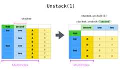
With a “stacked”DataFrame orSeries (having aMultiIndex as theindex), the inverse operation ofstack() isunstack(), which by defaultunstacks thelast level:
In [27]:stacked.unstack()Out[27]: A Bfirst secondbar one 0.895717 0.805244 two -1.206412 2.565646baz one 1.431256 1.340309 two -1.170299 -0.226169In [28]:stacked.unstack(1)Out[28]:second one twofirstbar A 0.895717 -1.206412 B 0.805244 2.565646baz A 1.431256 -1.170299 B 1.340309 -0.226169In [29]:stacked.unstack(0)Out[29]:first bar bazsecondone A 0.895717 1.431256 B 0.805244 1.340309two A -1.206412 -1.170299 B 2.565646 -0.226169
If the indexes have names, you can use the level names instead of specifyingthe level numbers:
In [30]:stacked.unstack("second")Out[30]:second one twofirstbar A 0.895717 -1.206412 B 0.805244 2.565646baz A 1.431256 -1.170299 B 1.340309 -0.226169
Notice that thestack() andunstack() methods implicitly sort the indexlevels involved. Hence a call tostack() and thenunstack(), or vice versa,will result in asorted copy of the originalDataFrame orSeries:
In [31]:index=pd.MultiIndex.from_product([[2,1],["a","b"]])In [32]:df=pd.DataFrame(np.random.randn(4),index=index,columns=["A"])In [33]:dfOut[33]: A2 a -1.413681 b 1.6079201 a 1.024180 b 0.569605In [34]:all(df.unstack().stack(future_stack=True)==df.sort_index())Out[34]:True
Multiple levels#
You may also stack or unstack more than one level at a time by passing a listof levels, in which case the end result is as if each level in the list wereprocessed individually.
In [35]:columns=pd.MultiIndex.from_tuples( ....:[ ....:("A","cat","long"), ....:("B","cat","long"), ....:("A","dog","short"), ....:("B","dog","short"), ....:], ....:names=["exp","animal","hair_length"], ....:) ....:In [36]:df=pd.DataFrame(np.random.randn(4,4),columns=columns)In [37]:dfOut[37]:exp A B A Banimal cat cat dog doghair_length long long short short0 0.875906 -2.211372 0.974466 -2.0067471 -0.410001 -0.078638 0.545952 -1.2192172 -1.226825 0.769804 -1.281247 -0.7277073 -0.121306 -0.097883 0.695775 0.341734In [38]:df.stack(level=["animal","hair_length"],future_stack=True)Out[38]:exp A B animal hair_length0 cat long 0.875906 -2.211372 dog short 0.974466 -2.0067471 cat long -0.410001 -0.078638 dog short 0.545952 -1.2192172 cat long -1.226825 0.769804 dog short -1.281247 -0.7277073 cat long -0.121306 -0.097883 dog short 0.695775 0.341734
The list of levels can contain either level names or level numbers butnot a mixture of the two.
# df.stack(level=['animal', 'hair_length'], future_stack=True)# from above is equivalent to:In [39]:df.stack(level=[1,2],future_stack=True)Out[39]:exp A B animal hair_length0 cat long 0.875906 -2.211372 dog short 0.974466 -2.0067471 cat long -0.410001 -0.078638 dog short 0.545952 -1.2192172 cat long -1.226825 0.769804 dog short -1.281247 -0.7277073 cat long -0.121306 -0.097883 dog short 0.695775 0.341734
Missing data#
Unstacking can result in missing values if subgroups do not have the sameset of labels. By default, missing values will be replaced with the defaultfill value for that data type.
In [40]:columns=pd.MultiIndex.from_tuples( ....:[ ....:("A","cat"), ....:("B","dog"), ....:("B","cat"), ....:("A","dog"), ....:], ....:names=["exp","animal"], ....:) ....:In [41]:index=pd.MultiIndex.from_product( ....:[("bar","baz","foo","qux"),("one","two")],names=["first","second"] ....:) ....:In [42]:df=pd.DataFrame(np.random.randn(8,4),index=index,columns=columns)In [43]:df3=df.iloc[[0,1,4,7],[1,2]]In [44]:df3Out[44]:exp Banimal dog catfirst secondbar one -1.110336 -0.619976 two 0.687738 0.176444foo one 1.314232 0.690579qux two 0.380396 0.084844In [45]:df3.unstack()Out[45]:exp Banimal dog catsecond one two one twofirstbar -1.110336 0.687738 -0.619976 0.176444foo 1.314232 NaN 0.690579 NaNqux NaN 0.380396 NaN 0.084844
The missing value can be filled with a specific value with thefill_value argument.
In [46]:df3.unstack(fill_value=-1e9)Out[46]:exp Banimal dog catsecond one two one twofirstbar -1.110336e+00 6.877384e-01 -6.199759e-01 1.764443e-01foo 1.314232e+00 -1.000000e+09 6.905793e-01 -1.000000e+09qux -1.000000e+09 3.803956e-01 -1.000000e+09 8.484421e-02
melt() andwide_to_long()#
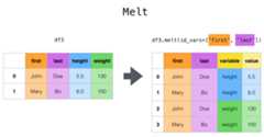
The top-levelmelt() function and the correspondingDataFrame.melt()are useful to massage aDataFrame into a format where one or more columnsareidentifier variables, while all other columns, consideredmeasuredvariables, are “unpivoted” to the row axis, leaving just two non-identifiercolumns, “variable” and “value”. The names of those columns can be customizedby supplying thevar_name andvalue_name parameters.
In [47]:cheese=pd.DataFrame( ....:{ ....:"first":["John","Mary"], ....:"last":["Doe","Bo"], ....:"height":[5.5,6.0], ....:"weight":[130,150], ....:} ....:) ....:In [48]:cheeseOut[48]: first last height weight0 John Doe 5.5 1301 Mary Bo 6.0 150In [49]:cheese.melt(id_vars=["first","last"])Out[49]: first last variable value0 John Doe height 5.51 Mary Bo height 6.02 John Doe weight 130.03 Mary Bo weight 150.0In [50]:cheese.melt(id_vars=["first","last"],var_name="quantity")Out[50]: first last quantity value0 John Doe height 5.51 Mary Bo height 6.02 John Doe weight 130.03 Mary Bo weight 150.0
When transforming a DataFrame usingmelt(), the index will be ignored.The original index values can be kept by setting theignore_index=False parameter toFalse (default isTrue).ignore_index=False will however duplicate index values.
In [51]:index=pd.MultiIndex.from_tuples([("person","A"),("person","B")])In [52]:cheese=pd.DataFrame( ....:{ ....:"first":["John","Mary"], ....:"last":["Doe","Bo"], ....:"height":[5.5,6.0], ....:"weight":[130,150], ....:}, ....:index=index, ....:) ....:In [53]:cheeseOut[53]: first last height weightperson A John Doe 5.5 130 B Mary Bo 6.0 150In [54]:cheese.melt(id_vars=["first","last"])Out[54]: first last variable value0 John Doe height 5.51 Mary Bo height 6.02 John Doe weight 130.03 Mary Bo weight 150.0In [55]:cheese.melt(id_vars=["first","last"],ignore_index=False)Out[55]: first last variable valueperson A John Doe height 5.5 B Mary Bo height 6.0 A John Doe weight 130.0 B Mary Bo weight 150.0
wide_to_long() is similar tomelt() with more customization forcolumn matching.
In [56]:dft=pd.DataFrame( ....:{ ....:"A1970":{0:"a",1:"b",2:"c"}, ....:"A1980":{0:"d",1:"e",2:"f"}, ....:"B1970":{0:2.5,1:1.2,2:0.7}, ....:"B1980":{0:3.2,1:1.3,2:0.1}, ....:"X":dict(zip(range(3),np.random.randn(3))), ....:} ....:) ....:In [57]:dft["id"]=dft.indexIn [58]:dftOut[58]: A1970 A1980 B1970 B1980 X id0 a d 2.5 3.2 1.519970 01 b e 1.2 1.3 -0.493662 12 c f 0.7 0.1 0.600178 2In [59]:pd.wide_to_long(dft,["A","B"],i="id",j="year")Out[59]: X A Bid year0 1970 1.519970 a 2.51 1970 -0.493662 b 1.22 1970 0.600178 c 0.70 1980 1.519970 d 3.21 1980 -0.493662 e 1.32 1980 0.600178 f 0.1
get_dummies() andfrom_dummies()#
To convert categorical variables of aSeries into a “dummy” or “indicator”,get_dummies() creates a newDataFrame with columns of the uniquevariables and the values representing the presence of those variables per row.
In [60]:df=pd.DataFrame({"key":list("bbacab"),"data1":range(6)})In [61]:pd.get_dummies(df["key"])Out[61]: a b c0 False True False1 False True False2 True False False3 False False True4 True False False5 False True FalseIn [62]:df["key"].str.get_dummies()Out[62]: a b c0 0 1 01 0 1 02 1 0 03 0 0 14 1 0 05 0 1 0
prefix adds a prefix to the the column names which is useful for merging the resultwith the originalDataFrame:
In [63]:dummies=pd.get_dummies(df["key"],prefix="key")In [64]:dummiesOut[64]: key_a key_b key_c0 False True False1 False True False2 True False False3 False False True4 True False False5 False True FalseIn [65]:df[["data1"]].join(dummies)Out[65]: data1 key_a key_b key_c0 0 False True False1 1 False True False2 2 True False False3 3 False False True4 4 True False False5 5 False True False
This function is often used along with discretization functions likecut():
In [66]:values=np.random.randn(10)In [67]:valuesOut[67]:array([ 0.2742, 0.1329, -0.0237, 2.4102, 1.4505, 0.2061, -0.2519, -2.2136, 1.0633, 1.2661])In [68]:bins=[0,0.2,0.4,0.6,0.8,1]In [69]:pd.get_dummies(pd.cut(values,bins))Out[69]: (0.0, 0.2] (0.2, 0.4] (0.4, 0.6] (0.6, 0.8] (0.8, 1.0]0 False True False False False1 True False False False False2 False False False False False3 False False False False False4 False False False False False5 False True False False False6 False False False False False7 False False False False False8 False False False False False9 False False False False False
get_dummies() also accepts aDataFrame. By default,object,string,orcategorical type columns are encoded as dummy variables with other columns unaltered.
In [70]:df=pd.DataFrame({"A":["a","b","a"],"B":["c","c","b"],"C":[1,2,3]})In [71]:pd.get_dummies(df)Out[71]: C A_a A_b B_b B_c0 1 True False False True1 2 False True False True2 3 True False True False
Specifying thecolumns keyword will encode a column of any type.
In [72]:pd.get_dummies(df,columns=["A"])Out[72]: B C A_a A_b0 c 1 True False1 c 2 False True2 b 3 True False
As with theSeries version, you can pass values for theprefix andprefix_sep. By default the column name is used as the prefix and_ asthe prefix separator. You can specifyprefix andprefix_sep in 3 ways:
string: Use the same value for
prefixorprefix_sepfor each columnto be encoded.list: Must be the same length as the number of columns being encoded.
dict: Mapping column name to prefix.
In [73]:simple=pd.get_dummies(df,prefix="new_prefix")In [74]:simpleOut[74]: C new_prefix_a new_prefix_b new_prefix_b new_prefix_c0 1 True False False True1 2 False True False True2 3 True False True FalseIn [75]:from_list=pd.get_dummies(df,prefix=["from_A","from_B"])In [76]:from_listOut[76]: C from_A_a from_A_b from_B_b from_B_c0 1 True False False True1 2 False True False True2 3 True False True FalseIn [77]:from_dict=pd.get_dummies(df,prefix={"B":"from_B","A":"from_A"})In [78]:from_dictOut[78]: C from_A_a from_A_b from_B_b from_B_c0 1 True False False True1 2 False True False True2 3 True False True False
To avoid collinearity when feeding the result to statistical models,specifydrop_first=True.
In [79]:s=pd.Series(list("abcaa"))In [80]:pd.get_dummies(s)Out[80]: a b c0 True False False1 False True False2 False False True3 True False False4 True False FalseIn [81]:pd.get_dummies(s,drop_first=True)Out[81]: b c0 False False1 True False2 False True3 False False4 False False
When a column contains only one level, it will be omitted in the result.
In [82]:df=pd.DataFrame({"A":list("aaaaa"),"B":list("ababc")})In [83]:pd.get_dummies(df)Out[83]: A_a B_a B_b B_c0 True True False False1 True False True False2 True True False False3 True False True False4 True False False TrueIn [84]:pd.get_dummies(df,drop_first=True)Out[84]: B_b B_c0 False False1 True False2 False False3 True False4 False True
The values can be cast to a different type using thedtype argument.
In [85]:df=pd.DataFrame({"A":list("abc"),"B":[1.1,2.2,3.3]})In [86]:pd.get_dummies(df,dtype=np.float32).dtypesOut[86]:B float64A_a float32A_b float32A_c float32dtype: object
Added in version 1.5.0.
from_dummies() converts the output ofget_dummies() back intoaSeries of categorical values from indicator values.
In [87]:df=pd.DataFrame({"prefix_a":[0,1,0],"prefix_b":[1,0,1]})In [88]:dfOut[88]: prefix_a prefix_b0 0 11 1 02 0 1In [89]:pd.from_dummies(df,sep="_")Out[89]: prefix0 b1 a2 b
Dummy coded data only requiresk-1 categories to be included, in this casethe last category is the default category. The default category can be modified withdefault_category.
In [90]:df=pd.DataFrame({"prefix_a":[0,1,0]})In [91]:dfOut[91]: prefix_a0 01 12 0In [92]:pd.from_dummies(df,sep="_",default_category="b")Out[92]: prefix0 b1 a2 b
explode()#
For aDataFrame column with nested, list-like values,explode() will transformeach list-like value to a separate row. The resultingIndex will be duplicated correspondingto the index label from the original row:
In [93]:keys=["panda1","panda2","panda3"]In [94]:values=[["eats","shoots"],["shoots","leaves"],["eats","leaves"]]In [95]:df=pd.DataFrame({"keys":keys,"values":values})In [96]:dfOut[96]: keys values0 panda1 [eats, shoots]1 panda2 [shoots, leaves]2 panda3 [eats, leaves]In [97]:df["values"].explode()Out[97]:0 eats0 shoots1 shoots1 leaves2 eats2 leavesName: values, dtype: object
DataFrame.explode can also explode the column in theDataFrame.
In [98]:df.explode("values")Out[98]: keys values0 panda1 eats0 panda1 shoots1 panda2 shoots1 panda2 leaves2 panda3 eats2 panda3 leaves
Series.explode() will replace empty lists with a missing value indicator and preserve scalar entries.
In [99]:s=pd.Series([[1,2,3],"foo",[],["a","b"]])In [100]:sOut[100]:0 [1, 2, 3]1 foo2 []3 [a, b]dtype: objectIn [101]:s.explode()Out[101]:0 10 20 31 foo2 NaN3 a3 bdtype: object
A comma-separated string value can be split into individual values in a list and then exploded to a new row.
In [102]:df=pd.DataFrame([{"var1":"a,b,c","var2":1},{"var1":"d,e,f","var2":2}])In [103]:df.assign(var1=df.var1.str.split(",")).explode("var1")Out[103]: var1 var20 a 10 b 10 c 11 d 21 e 21 f 2
crosstab()#
Usecrosstab() to compute a cross-tabulation of two (or more)factors. By defaultcrosstab() computes a frequency table of the factorsunless an array of values and an aggregation function are passed.
AnySeries passed will have their name attributes used unless row or columnnames for the cross-tabulation are specified
In [104]:a=np.array(["foo","foo","bar","bar","foo","foo"],dtype=object)In [105]:b=np.array(["one","one","two","one","two","one"],dtype=object)In [106]:c=np.array(["dull","dull","shiny","dull","dull","shiny"],dtype=object)In [107]:pd.crosstab(a,[b,c],rownames=["a"],colnames=["b","c"])Out[107]:b one twoc dull shiny dull shinyabar 1 0 0 1foo 2 1 1 0
Ifcrosstab() receives only twoSeries, it will provide a frequency table.
In [108]:df=pd.DataFrame( .....:{"A":[1,2,2,2,2],"B":[3,3,4,4,4],"C":[1,1,np.nan,1,1]} .....:) .....:In [109]:dfOut[109]: A B C0 1 3 1.01 2 3 1.02 2 4 NaN3 2 4 1.04 2 4 1.0In [110]:pd.crosstab(df["A"],df["B"])Out[110]:B 3 4A1 1 02 1 3
crosstab() can also summarize toCategorical data.
In [111]:foo=pd.Categorical(["a","b"],categories=["a","b","c"])In [112]:bar=pd.Categorical(["d","e"],categories=["d","e","f"])In [113]:pd.crosstab(foo,bar)Out[113]:col_0 d erow_0a 1 0b 0 1
ForCategorical data, to includeall of data categories even if the actual data doesnot contain any instances of a particular category, usedropna=False.
In [114]:pd.crosstab(foo,bar,dropna=False)Out[114]:col_0 d e frow_0a 1 0 0b 0 1 0c 0 0 0
Normalization#
Frequency tables can also be normalized to show percentages rather than countsusing thenormalize argument:
In [115]:pd.crosstab(df["A"],df["B"],normalize=True)Out[115]:B 3 4A1 0.2 0.02 0.2 0.6
normalize can also normalize values within each row or within each column:
In [116]:pd.crosstab(df["A"],df["B"],normalize="columns")Out[116]:B 3 4A1 0.5 0.02 0.5 1.0
crosstab() can also accept a thirdSeries and an aggregation function(aggfunc) that will be applied to the values of the thirdSeries withineach group defined by the first twoSeries:
In [117]:pd.crosstab(df["A"],df["B"],values=df["C"],aggfunc="sum")Out[117]:B 3 4A1 1.0 NaN2 1.0 2.0
Adding margins#
margins=True will add a row and column with anAll label with partial group aggregatesacross the categories on the rows and columns:
In [118]:pd.crosstab( .....:df["A"],df["B"],values=df["C"],aggfunc="sum",normalize=True,margins=True .....:) .....:Out[118]:B 3 4 AllA1 0.25 0.0 0.252 0.25 0.5 0.75All 0.50 0.5 1.00
cut()#
Thecut() function computes groupings for the values of the inputarray and is often used to transform continuous variables to discrete orcategorical variables:
An integerbins will form equal-width bins.
In [119]:ages=np.array([10,15,13,12,23,25,28,59,60])In [120]:pd.cut(ages,bins=3)Out[120]:[(9.95, 26.667], (9.95, 26.667], (9.95, 26.667], (9.95, 26.667], (9.95, 26.667], (9.95, 26.667], (26.667, 43.333], (43.333, 60.0], (43.333, 60.0]]Categories (3, interval[float64, right]): [(9.95, 26.667] < (26.667, 43.333] < (43.333, 60.0]]
A list of ordered bin edges will assign an interval for each variable.
In [121]:pd.cut(ages,bins=[0,18,35,70])Out[121]:[(0, 18], (0, 18], (0, 18], (0, 18], (18, 35], (18, 35], (18, 35], (35, 70], (35, 70]]Categories (3, interval[int64, right]): [(0, 18] < (18, 35] < (35, 70]]
If thebins keyword is anIntervalIndex, then these will beused to bin the passed data.
In [122]:pd.cut(ages,bins=pd.IntervalIndex.from_breaks([0,40,70]))Out[122]:[(0, 40], (0, 40], (0, 40], (0, 40], (0, 40], (0, 40], (0, 40], (40, 70], (40, 70]]Categories (2, interval[int64, right]): [(0, 40] < (40, 70]]
factorize()#
factorize() encodes 1 dimensional values into integer labels. Missing valuesare encoded as-1.
In [123]:x=pd.Series(["A","A",np.nan,"B",3.14,np.inf])In [124]:xOut[124]:0 A1 A2 NaN3 B4 3.145 infdtype: objectIn [125]:labels,uniques=pd.factorize(x)In [126]:labelsOut[126]:array([ 0, 0, -1, 1, 2, 3])In [127]:uniquesOut[127]:Index(['A', 'B', 3.14, inf], dtype='object')
Categorical will similarly encode 1 dimensional values for furthercategorical operations
In [128]:pd.Categorical(x)Out[128]:['A', 'A', NaN, 'B', 3.14, inf]Categories (4, object): [3.14, inf, 'A', 'B']