Group by: split-apply-combine#
By “group by” we are referring to a process involving one or more of the followingsteps:
Splitting the data into groups based on some criteria.
Applying a function to each group independently.
Combining the results into a data structure.
Out of these, the split step is the most straightforward. In the apply step, wemight wish to do one of the following:
Aggregation: compute a summary statistic (or statistics) for eachgroup. Some examples:
Compute group sums or means.
Compute group sizes / counts.
Transformation: perform some group-specific computations and return alike-indexed object. Some examples:
Standardize data (zscore) within a group.
Filling NAs within groups with a value derived from each group.
Filtration: discard some groups, according to a group-wise computationthat evaluates to True or False. Some examples:
Discard data that belong to groups with only a few members.
Filter out data based on the group sum or mean.
Many of these operations are defined on GroupBy objects. These operations are similarto those of theaggregating API,window API, andresample API.
It is possible that a given operation does not fall into one of these categories oris some combination of them. In such a case, it may be possible to compute theoperation using GroupBy’sapply method. This method will examine the results of theapply step and try to sensibly combine them into a single result if it doesn’t fit into eitherof the above three categories.
Note
An operation that is split into multiple steps using built-in GroupBy operationswill be more efficient than using theapply method with a user-defined Pythonfunction.
The name GroupBy should be quite familiar to those who have useda SQL-based tool (oritertools), in which you can write code like:
SELECTColumn1,Column2,mean(Column3),sum(Column4)FROMSomeTableGROUPBYColumn1,Column2
We aim to make operations like this natural and easy to express usingpandas. We’ll address each area of GroupBy functionality, then provide somenon-trivial examples / use cases.
See thecookbook for some advanced strategies.
Splitting an object into groups#
The abstract definition of grouping is to provide a mapping of labels togroup names. To create a GroupBy object (more on what the GroupBy object islater), you may do the following:
In [1]:speeds=pd.DataFrame( ...:[ ...:("bird","Falconiformes",389.0), ...:("bird","Psittaciformes",24.0), ...:("mammal","Carnivora",80.2), ...:("mammal","Primates",np.nan), ...:("mammal","Carnivora",58), ...:], ...:index=["falcon","parrot","lion","monkey","leopard"], ...:columns=("class","order","max_speed"), ...:) ...:In [2]:speedsOut[2]: class order max_speedfalcon bird Falconiformes 389.0parrot bird Psittaciformes 24.0lion mammal Carnivora 80.2monkey mammal Primates NaNleopard mammal Carnivora 58.0In [3]:grouped=speeds.groupby("class")In [4]:grouped=speeds.groupby(["class","order"])
The mapping can be specified many different ways:
A Python function, to be called on each of the index labels.
A list or NumPy array of the same length as the index.
A dict or
Series, providing alabel->groupnamemapping.For
DataFrameobjects, a string indicating either a column name oran index level name to be used to group.A list of any of the above things.
Collectively we refer to the grouping objects as thekeys. For example,consider the followingDataFrame:
Note
A string passed togroupby may refer to either a column or an index level.If a string matches both a column name and an index level name, aValueError will be raised.
In [5]:df=pd.DataFrame( ...:{ ...:"A":["foo","bar","foo","bar","foo","bar","foo","foo"], ...:"B":["one","one","two","three","two","two","one","three"], ...:"C":np.random.randn(8), ...:"D":np.random.randn(8), ...:} ...:) ...:In [6]:dfOut[6]: A B C D0 foo one 0.469112 -0.8618491 bar one -0.282863 -2.1045692 foo two -1.509059 -0.4949293 bar three -1.135632 1.0718044 foo two 1.212112 0.7215555 bar two -0.173215 -0.7067716 foo one 0.119209 -1.0395757 foo three -1.044236 0.271860
On a DataFrame, we obtain a GroupBy object by callinggroupby().This method returns apandas.api.typing.DataFrameGroupBy instance.We could naturally group by either theA orB columns, or both:
In [7]:grouped=df.groupby("A")In [8]:grouped=df.groupby("B")In [9]:grouped=df.groupby(["A","B"])
Note
df.groupby('A') is just syntactic sugar fordf.groupby(df['A']).
If we also have a MultiIndex on columnsA andB, we can group by allthe columns except the one we specify:
In [10]:df2=df.set_index(["A","B"])In [11]:grouped=df2.groupby(level=df2.index.names.difference(["B"]))In [12]:grouped.sum()Out[12]: C DAbar -1.591710 -1.739537foo -0.752861 -1.402938
The above GroupBy will split the DataFrame on its index (rows). To split by columns, first doa transpose:
In [13]:defget_letter_type(letter): ....:ifletter.lower()in'aeiou': ....:return'vowel' ....:else: ....:return'consonant' ....:In [14]:grouped=df.T.groupby(get_letter_type)
pandasIndex objects support duplicate values. If anon-unique index is used as the group key in a groupby operation, all valuesfor the same index value will be considered to be in one group and thus theoutput of aggregation functions will only contain unique index values:
In [15]:index=[1,2,3,1,2,3]In [16]:s=pd.Series([1,2,3,10,20,30],index=index)In [17]:sOut[17]:1 12 23 31 102 203 30dtype: int64In [18]:grouped=s.groupby(level=0)In [19]:grouped.first()Out[19]:1 12 23 3dtype: int64In [20]:grouped.last()Out[20]:1 102 203 30dtype: int64In [21]:grouped.sum()Out[21]:1 112 223 33dtype: int64
Note thatno splitting occurs until it’s needed. Creating the GroupBy objectonly verifies that you’ve passed a valid mapping.
Note
Many kinds of complicated data manipulations can be expressed in terms ofGroupBy operations (though it can’t be guaranteed to be the most efficient implementation).You can get quite creative with the label mapping functions.
GroupBy sorting#
By default the group keys are sorted during thegroupby operation. You may however passsort=False for potential speedups. Withsort=False the order among group-keys follows the order of appearance of the keys in the original dataframe:
In [22]:df2=pd.DataFrame({"X":["B","B","A","A"],"Y":[1,2,3,4]})In [23]:df2.groupby(["X"]).sum()Out[23]: YXA 7B 3In [24]:df2.groupby(["X"],sort=False).sum()Out[24]: YXB 3A 7
Note thatgroupby will preserve the order in whichobservations are sortedwithin each group.For example, the groups created bygroupby() below are in the order they appeared in the originalDataFrame:
In [25]:df3=pd.DataFrame({"X":["A","B","A","B"],"Y":[1,4,3,2]})In [26]:df3.groupby("X").get_group("A")Out[26]: X Y0 A 12 A 3In [27]:df3.groupby(["X"]).get_group(("B",))Out[27]: X Y1 B 43 B 2
GroupBy dropna#
By defaultNA values are excluded from group keys during thegroupby operation. However,in case you want to includeNA values in group keys, you could passdropna=False to achieve it.
In [28]:df_list=[[1,2,3],[1,None,4],[2,1,3],[1,2,2]]In [29]:df_dropna=pd.DataFrame(df_list,columns=["a","b","c"])In [30]:df_dropnaOut[30]: a b c0 1 2.0 31 1 NaN 42 2 1.0 33 1 2.0 2
# Default ``dropna`` is set to True, which will exclude NaNs in keysIn [31]:df_dropna.groupby(by=["b"],dropna=True).sum()Out[31]: a cb1.0 2 32.0 2 5# In order to allow NaN in keys, set ``dropna`` to FalseIn [32]:df_dropna.groupby(by=["b"],dropna=False).sum()Out[32]: a cb1.0 2 32.0 2 5NaN 1 4
The default setting ofdropna argument isTrue which meansNA are not included in group keys.
GroupBy object attributes#
Thegroups attribute is a dictionary whose keys are the computed unique groupsand corresponding values are the axis labels belonging to each group. In theabove example we have:
In [33]:df.groupby("A").groupsOut[33]:{'bar': [1, 3, 5], 'foo': [0, 2, 4, 6, 7]}In [34]:df.T.groupby(get_letter_type).groupsOut[34]:{'consonant': ['B', 'C', 'D'], 'vowel': ['A']}
Calling the standard Pythonlen function on the GroupBy object returnsthe number of groups, which is the same as the length of thegroups dictionary:
In [35]:grouped=df.groupby(["A","B"])In [36]:grouped.groupsOut[36]:{('bar', 'one'): [1], ('bar', 'three'): [3], ('bar', 'two'): [5], ('foo', 'one'): [0, 6], ('foo', 'three'): [7], ('foo', 'two'): [2, 4]}In [37]:len(grouped)Out[37]:6
GroupBy will tab complete column names, GroupBy operations, and other attributes:
In [38]:n=10In [39]:weight=np.random.normal(166,20,size=n)In [40]:height=np.random.normal(60,10,size=n)In [41]:time=pd.date_range("1/1/2000",periods=n)In [42]:gender=np.random.choice(["male","female"],size=n)In [43]:df=pd.DataFrame( ....:{"height":height,"weight":weight,"gender":gender},index=time ....:) ....:In [44]:dfOut[44]: height weight gender2000-01-01 42.849980 157.500553 male2000-01-02 49.607315 177.340407 male2000-01-03 56.293531 171.524640 male2000-01-04 48.421077 144.251986 female2000-01-05 46.556882 152.526206 male2000-01-06 68.448851 168.272968 female2000-01-07 70.757698 136.431469 male2000-01-08 58.909500 176.499753 female2000-01-09 76.435631 174.094104 female2000-01-10 45.306120 177.540920 maleIn [45]:gb=df.groupby("gender")
In [46]:gb.<TAB># noqa: E225, E999gb.agg gb.boxplot gb.cummin gb.describe gb.filter gb.get_group gb.height gb.last gb.median gb.ngroups gb.plot gb.rank gb.std gb.transformgb.aggregate gb.count gb.cumprod gb.dtype gb.first gb.groups gb.hist gb.max gb.min gb.nth gb.prod gb.resample gb.sum gb.vargb.apply gb.cummax gb.cumsum gb.fillna gb.gender gb.head gb.indices gb.mean gb.name gb.ohlc gb.quantile gb.size gb.tail gb.weight
GroupBy with MultiIndex#
Withhierarchically-indexed data, it’s quitenatural to group by one of the levels of the hierarchy.
Let’s create a Series with a two-levelMultiIndex.
In [47]:arrays=[ ....:["bar","bar","baz","baz","foo","foo","qux","qux"], ....:["one","two","one","two","one","two","one","two"], ....:] ....:In [48]:index=pd.MultiIndex.from_arrays(arrays,names=["first","second"])In [49]:s=pd.Series(np.random.randn(8),index=index)In [50]:sOut[50]:first secondbar one -0.919854 two -0.042379baz one 1.247642 two -0.009920foo one 0.290213 two 0.495767qux one 0.362949 two 1.548106dtype: float64
We can then group by one of the levels ins.
In [51]:grouped=s.groupby(level=0)In [52]:grouped.sum()Out[52]:firstbar -0.962232baz 1.237723foo 0.785980qux 1.911055dtype: float64
If the MultiIndex has names specified, these can be passed instead of the levelnumber:
In [53]:s.groupby(level="second").sum()Out[53]:secondone 0.980950two 1.991575dtype: float64
Grouping with multiple levels is supported.
In [54]:arrays=[ ....:["bar","bar","baz","baz","foo","foo","qux","qux"], ....:["doo","doo","bee","bee","bop","bop","bop","bop"], ....:["one","two","one","two","one","two","one","two"], ....:] ....:In [55]:index=pd.MultiIndex.from_arrays(arrays,names=["first","second","third"])In [56]:s=pd.Series(np.random.randn(8),index=index)In [57]:sOut[57]:first second thirdbar doo one -1.131345 two -0.089329baz bee one 0.337863 two -0.945867foo bop one -0.932132 two 1.956030qux bop one 0.017587 two -0.016692dtype: float64In [58]:s.groupby(level=["first","second"]).sum()Out[58]:first secondbar doo -1.220674baz bee -0.608004foo bop 1.023898qux bop 0.000895dtype: float64
Index level names may be supplied as keys.
In [59]:s.groupby(["first","second"]).sum()Out[59]:first secondbar doo -1.220674baz bee -0.608004foo bop 1.023898qux bop 0.000895dtype: float64
More on thesum function and aggregation later.
Grouping DataFrame with Index levels and columns#
A DataFrame may be grouped by a combination of columns and index levels. Youcan specify both column and index names, or use aGrouper.
Let’s first create a DataFrame with a MultiIndex:
In [60]:arrays=[ ....:["bar","bar","baz","baz","foo","foo","qux","qux"], ....:["one","two","one","two","one","two","one","two"], ....:] ....:In [61]:index=pd.MultiIndex.from_arrays(arrays,names=["first","second"])In [62]:df=pd.DataFrame({"A":[1,1,1,1,2,2,3,3],"B":np.arange(8)},index=index)In [63]:dfOut[63]: A Bfirst secondbar one 1 0 two 1 1baz one 1 2 two 1 3foo one 2 4 two 2 5qux one 3 6 two 3 7
Then we groupdf by thesecond index level and theA column.
In [64]:df.groupby([pd.Grouper(level=1),"A"]).sum()Out[64]: Bsecond Aone 1 2 2 4 3 6two 1 4 2 5 3 7
Index levels may also be specified by name.
In [65]:df.groupby([pd.Grouper(level="second"),"A"]).sum()Out[65]: Bsecond Aone 1 2 2 4 3 6two 1 4 2 5 3 7
Index level names may be specified as keys directly togroupby.
In [66]:df.groupby(["second","A"]).sum()Out[66]: Bsecond Aone 1 2 2 4 3 6two 1 4 2 5 3 7
DataFrame column selection in GroupBy#
Once you have created the GroupBy object from a DataFrame, you might want to dosomething different for each of the columns. Thus, by using[] on the GroupByobject in a similar way as the one used to get a column from a DataFrame, you can do:
In [67]:df=pd.DataFrame( ....:{ ....:"A":["foo","bar","foo","bar","foo","bar","foo","foo"], ....:"B":["one","one","two","three","two","two","one","three"], ....:"C":np.random.randn(8), ....:"D":np.random.randn(8), ....:} ....:) ....:In [68]:dfOut[68]: A B C D0 foo one -0.575247 1.3460611 bar one 0.254161 1.5117632 foo two -1.143704 1.6270813 bar three 0.215897 -0.9905824 foo two 1.193555 -0.4416525 bar two -0.077118 1.2115266 foo one -0.408530 0.2685207 foo three -0.862495 0.024580In [69]:grouped=df.groupby(["A"])In [70]:grouped_C=grouped["C"]In [71]:grouped_D=grouped["D"]
This is mainly syntactic sugar for the alternative, which is much more verbose:
In [72]:df["C"].groupby(df["A"])Out[72]:<pandas.core.groupby.generic.SeriesGroupBy object at 0x7f945c0eacb0>
Additionally, this method avoids recomputing the internal grouping informationderived from the passed key.
You can also include the grouping columns if you want to operate on them.
In [73]:grouped[["A","B"]].sum()Out[73]: A BAbar barbarbar onethreetwofoo foofoofoofoofoo onetwotwoonethree
Iterating through groups#
With the GroupBy object in hand, iterating through the grouped data is verynatural and functions similarly toitertools.groupby():
In [74]:grouped=df.groupby('A')In [75]:forname,groupingrouped: ....:print(name) ....:print(group) ....:bar A B C D1 bar one 0.254161 1.5117633 bar three 0.215897 -0.9905825 bar two -0.077118 1.211526foo A B C D0 foo one -0.575247 1.3460612 foo two -1.143704 1.6270814 foo two 1.193555 -0.4416526 foo one -0.408530 0.2685207 foo three -0.862495 0.024580
In the case of grouping by multiple keys, the group name will be a tuple:
In [76]:forname,groupindf.groupby(['A','B']): ....:print(name) ....:print(group) ....:('bar', 'one') A B C D1 bar one 0.254161 1.511763('bar', 'three') A B C D3 bar three 0.215897 -0.990582('bar', 'two') A B C D5 bar two -0.077118 1.211526('foo', 'one') A B C D0 foo one -0.575247 1.3460616 foo one -0.408530 0.268520('foo', 'three') A B C D7 foo three -0.862495 0.02458('foo', 'two') A B C D2 foo two -1.143704 1.6270814 foo two 1.193555 -0.441652
Selecting a group#
A single group can be selected usingDataFrameGroupBy.get_group():
In [77]:grouped.get_group("bar")Out[77]: A B C D1 bar one 0.254161 1.5117633 bar three 0.215897 -0.9905825 bar two -0.077118 1.211526
Or for an object grouped on multiple columns:
In [78]:df.groupby(["A","B"]).get_group(("bar","one"))Out[78]: A B C D1 bar one 0.254161 1.511763
Aggregation#
An aggregation is a GroupBy operation that reduces the dimension of the groupingobject. The result of an aggregation is, or at least is treated as,a scalar value for each column in a group. For example, producing the sum of eachcolumn in a group of values.
In [79]:animals=pd.DataFrame( ....:{ ....:"kind":["cat","dog","cat","dog"], ....:"height":[9.1,6.0,9.5,34.0], ....:"weight":[7.9,7.5,9.9,198.0], ....:} ....:) ....:In [80]:animalsOut[80]: kind height weight0 cat 9.1 7.91 dog 6.0 7.52 cat 9.5 9.93 dog 34.0 198.0In [81]:animals.groupby("kind").sum()Out[81]: height weightkindcat 18.6 17.8dog 40.0 205.5
In the result, the keys of the groups appear in the index by default. They can beinstead included in the columns by passingas_index=False.
In [82]:animals.groupby("kind",as_index=False).sum()Out[82]: kind height weight0 cat 18.6 17.81 dog 40.0 205.5
Built-in aggregation methods#
Many common aggregations are built-in to GroupBy objects as methods. Of the methodslisted below, those with a* donot have an efficient, GroupBy-specific, implementation.
Method | Description |
|---|---|
Compute whether any of the values in the groups are truthy | |
Compute whether all of the values in the groups are truthy | |
Compute the number of non-NA values in the groups | |
| Compute the covariance of the groups |
Compute the first occurring value in each group | |
Compute the index of the maximum value in each group | |
Compute the index of the minimum value in each group | |
Compute the last occurring value in each group | |
Compute the maximum value in each group | |
Compute the mean of each group | |
Compute the median of each group | |
Compute the minimum value in each group | |
Compute the number of unique values in each group | |
Compute the product of the values in each group | |
Compute a given quantile of the values in each group | |
Compute the standard error of the mean of the values in each group | |
Compute the number of values in each group | |
| Compute the skew of the values in each group |
Compute the standard deviation of the values in each group | |
Compute the sum of the values in each group | |
Compute the variance of the values in each group |
Some examples:
In [83]:df.groupby("A")[["C","D"]].max()Out[83]: C DAbar 0.254161 1.511763foo 1.193555 1.627081In [84]:df.groupby(["A","B"]).mean()Out[84]: C DA Bbar one 0.254161 1.511763 three 0.215897 -0.990582 two -0.077118 1.211526foo one -0.491888 0.807291 three -0.862495 0.024580 two 0.024925 0.592714
Another aggregation example is to compute the size of each group.This is included in GroupBy as thesize method. It returns a Series whoseindex consists of the group names and the values are the sizes of each group.
In [85]:grouped=df.groupby(["A","B"])In [86]:grouped.size()Out[86]:A Bbar one 1 three 1 two 1foo one 2 three 1 two 2dtype: int64
While theDataFrameGroupBy.describe() method is not itself a reducer, itcan be used to conveniently produce a collection of summary statistics about each ofthe groups.
In [87]:grouped.describe()Out[87]: C ... D count mean std ... 50% 75% maxA B ...bar one 1.0 0.254161 NaN ... 1.511763 1.511763 1.511763 three 1.0 0.215897 NaN ... -0.990582 -0.990582 -0.990582 two 1.0 -0.077118 NaN ... 1.211526 1.211526 1.211526foo one 2.0 -0.491888 0.117887 ... 0.807291 1.076676 1.346061 three 1.0 -0.862495 NaN ... 0.024580 0.024580 0.024580 two 2.0 0.024925 1.652692 ... 0.592714 1.109898 1.627081[6 rows x 16 columns]
Another aggregation example is to compute the number of unique values of each group.This is similar to theDataFrameGroupBy.value_counts() function, except that it only counts thenumber of unique values.
In [88]:ll=[['foo',1],['foo',2],['foo',2],['bar',1],['bar',1]]In [89]:df4=pd.DataFrame(ll,columns=["A","B"])In [90]:df4Out[90]: A B0 foo 11 foo 22 foo 23 bar 14 bar 1In [91]:df4.groupby("A")["B"].nunique()Out[91]:Abar 1foo 2Name: B, dtype: int64
Note
Aggregation functionswill not return the groups that you are aggregating overas namedcolumns whenas_index=True, the default. The grouped columns willbe theindices of the returned object.
Passingas_index=Falsewill return the groups that you are aggregating over asnamed columns, regardless if they are namedindices orcolumns in the inputs.
Theaggregate() method#
Note
Theaggregate() method can accept many different types ofinputs. This section details using string aliases for various GroupBy methods; otherinputs are detailed in the sections below.
Any reduction method that pandas implements can be passed as a string toaggregate(). Users are encouraged to use the shorthand,agg. It will operate as if the corresponding method was called.
In [92]:grouped=df.groupby("A")In [93]:grouped[["C","D"]].aggregate("sum")Out[93]: C DAbar 0.392940 1.732707foo -1.796421 2.824590In [94]:grouped=df.groupby(["A","B"])In [95]:grouped.agg("sum")Out[95]: C DA Bbar one 0.254161 1.511763 three 0.215897 -0.990582 two -0.077118 1.211526foo one -0.983776 1.614581 three -0.862495 0.024580 two 0.049851 1.185429
The result of the aggregation will have the group names as thenew index. In the case of multiple keys, the result is aMultiIndex by default. As mentioned above, this can bechanged by using theas_index option:
In [96]:grouped=df.groupby(["A","B"],as_index=False)In [97]:grouped.agg("sum")Out[97]: A B C D0 bar one 0.254161 1.5117631 bar three 0.215897 -0.9905822 bar two -0.077118 1.2115263 foo one -0.983776 1.6145814 foo three -0.862495 0.0245805 foo two 0.049851 1.185429In [98]:df.groupby("A",as_index=False)[["C","D"]].agg("sum")Out[98]: A C D0 bar 0.392940 1.7327071 foo -1.796421 2.824590
Note that you could use theDataFrame.reset_index() DataFrame function to achievethe same result as the column names are stored in the resultingMultiIndex, althoughthis will make an extra copy.
In [99]:df.groupby(["A","B"]).agg("sum").reset_index()Out[99]: A B C D0 bar one 0.254161 1.5117631 bar three 0.215897 -0.9905822 bar two -0.077118 1.2115263 foo one -0.983776 1.6145814 foo three -0.862495 0.0245805 foo two 0.049851 1.185429
Aggregation with User-Defined Functions#
Users can also provide their own User-Defined Functions (UDFs) for custom aggregations.
Warning
When aggregating with a UDF, the UDF should not mutate theprovidedSeries. SeeMutating with User Defined Function (UDF) methods for more information.
Note
Aggregating with a UDF is often less performant than usingthe pandas built-in methods on GroupBy. Consider breaking up a complex operationinto a chain of operations that utilize the built-in methods.
In [100]:animalsOut[100]: kind height weight0 cat 9.1 7.91 dog 6.0 7.52 cat 9.5 9.93 dog 34.0 198.0In [101]:animals.groupby("kind")[["height"]].agg(lambdax:set(x))Out[101]: heightkindcat {9.1, 9.5}dog {34.0, 6.0}
The resulting dtype will reflect that of the aggregating function. If the results from different groups havedifferent dtypes, then a common dtype will be determined in the same way asDataFrame construction.
In [102]:animals.groupby("kind")[["height"]].agg(lambdax:x.astype(int).sum())Out[102]: heightkindcat 18dog 40
Applying multiple functions at once#
On a groupedSeries, you can pass a list or dict of functions toSeriesGroupBy.agg(), outputting a DataFrame:
In [103]:grouped=df.groupby("A")In [104]:grouped["C"].agg(["sum","mean","std"])Out[104]: sum mean stdAbar 0.392940 0.130980 0.181231foo -1.796421 -0.359284 0.912265
On a groupedDataFrame, you can pass a list of functions toDataFrameGroupBy.agg() to aggregate eachcolumn, which produces an aggregated result with a hierarchical column index:
In [105]:grouped[["C","D"]].agg(["sum","mean","std"])Out[105]: C D sum mean std sum mean stdAbar 0.392940 0.130980 0.181231 1.732707 0.577569 1.366330foo -1.796421 -0.359284 0.912265 2.824590 0.564918 0.884785
The resulting aggregations are named after the functions themselves. If youneed to rename, then you can add in a chained operation for aSeries like this:
In [106]:( .....:grouped["C"] .....:.agg(["sum","mean","std"]) .....:.rename(columns={"sum":"foo","mean":"bar","std":"baz"}) .....:) .....:Out[106]: foo bar bazAbar 0.392940 0.130980 0.181231foo -1.796421 -0.359284 0.912265
For a groupedDataFrame, you can rename in a similar manner:
In [107]:( .....:grouped[["C","D"]].agg(["sum","mean","std"]).rename( .....:columns={"sum":"foo","mean":"bar","std":"baz"} .....:) .....:) .....:Out[107]: C D foo bar baz foo bar bazAbar 0.392940 0.130980 0.181231 1.732707 0.577569 1.366330foo -1.796421 -0.359284 0.912265 2.824590 0.564918 0.884785
Note
In general, the output column names should be unique, but pandas will allowyou apply to the same function (or two functions with the same name) to the samecolumn.
In [108]:grouped["C"].agg(["sum","sum"])Out[108]: sum sumAbar 0.392940 0.392940foo -1.796421 -1.796421
pandas also allows you to provide multiple lambdas. In this case, pandaswill mangle the name of the (nameless) lambda functions, appending_<i>to each subsequent lambda.
In [109]:grouped["C"].agg([lambdax:x.max()-x.min(),lambdax:x.median()-x.mean()])Out[109]: <lambda_0> <lambda_1>Abar 0.331279 0.084917foo 2.337259 -0.215962
Named aggregation#
To support column-specific aggregationwith control over the output column names, pandasaccepts the special syntax inDataFrameGroupBy.agg() andSeriesGroupBy.agg(), known as “named aggregation”, where
The keywords are theoutput column names
The values are tuples whose first element is the column to selectand the second element is the aggregation to apply to that column. pandasprovides the
NamedAggnamedtuple with the fields['column','aggfunc']to make it clearer what the arguments are. As usual, the aggregation canbe a callable or a string alias.
In [110]:animalsOut[110]: kind height weight0 cat 9.1 7.91 dog 6.0 7.52 cat 9.5 9.93 dog 34.0 198.0In [111]:animals.groupby("kind").agg( .....:min_height=pd.NamedAgg(column="height",aggfunc="min"), .....:max_height=pd.NamedAgg(column="height",aggfunc="max"), .....:average_weight=pd.NamedAgg(column="weight",aggfunc="mean"), .....:) .....:Out[111]: min_height max_height average_weightkindcat 9.1 9.5 8.90dog 6.0 34.0 102.75
NamedAgg is just anamedtuple. Plain tuples are allowed as well.
In [112]:animals.groupby("kind").agg( .....:min_height=("height","min"), .....:max_height=("height","max"), .....:average_weight=("weight","mean"), .....:) .....:Out[112]: min_height max_height average_weightkindcat 9.1 9.5 8.90dog 6.0 34.0 102.75
If the column names you want are not valid Python keywords, construct a dictionaryand unpack the keyword arguments
In [113]:animals.groupby("kind").agg( .....:**{ .....:"total weight":pd.NamedAgg(column="weight",aggfunc="sum") .....:} .....:) .....:Out[113]: total weightkindcat 17.8dog 205.5
When using named aggregation, additional keyword arguments are not passed throughto the aggregation functions; only pairsof(column,aggfunc) should be passed as**kwargs. If your aggregation functionsrequire additional arguments, apply them partially withfunctools.partial().
Named aggregation is also valid for Series groupby aggregations. In this case there’sno column selection, so the values are just the functions.
In [114]:animals.groupby("kind").height.agg( .....:min_height="min", .....:max_height="max", .....:) .....:Out[114]: min_height max_heightkindcat 9.1 9.5dog 6.0 34.0
Applying different functions to DataFrame columns#
By passing a dict toaggregate you can apply a different aggregation to thecolumns of a DataFrame:
In [115]:grouped.agg({"C":"sum","D":lambdax:np.std(x,ddof=1)})Out[115]: C DAbar 0.392940 1.366330foo -1.796421 0.884785
The function names can also be strings. In order for a string to be valid itmust be implemented on GroupBy:
In [116]:grouped.agg({"C":"sum","D":"std"})Out[116]: C DAbar 0.392940 1.366330foo -1.796421 0.884785
Transformation#
A transformation is a GroupBy operation whose result is indexed the sameas the one being grouped. Common examples includecumsum() anddiff().
In [117]:speedsOut[117]: class order max_speedfalcon bird Falconiformes 389.0parrot bird Psittaciformes 24.0lion mammal Carnivora 80.2monkey mammal Primates NaNleopard mammal Carnivora 58.0In [118]:grouped=speeds.groupby("class")["max_speed"]In [119]:grouped.cumsum()Out[119]:falcon 389.0parrot 413.0lion 80.2monkey NaNleopard 138.2Name: max_speed, dtype: float64In [120]:grouped.diff()Out[120]:falcon NaNparrot -365.0lion NaNmonkey NaNleopard NaNName: max_speed, dtype: float64
Unlike aggregations, the groupings that are used to splitthe original object are not included in the result.
Note
Since transformations do not include the groupings that are used to split the result,the argumentsas_index andsort inDataFrame.groupby() andSeries.groupby() have no effect.
A common use of a transformation is to add the result back into the original DataFrame.
In [121]:result=speeds.copy()In [122]:result["cumsum"]=grouped.cumsum()In [123]:result["diff"]=grouped.diff()In [124]:resultOut[124]: class order max_speed cumsum difffalcon bird Falconiformes 389.0 389.0 NaNparrot bird Psittaciformes 24.0 413.0 -365.0lion mammal Carnivora 80.2 80.2 NaNmonkey mammal Primates NaN NaN NaNleopard mammal Carnivora 58.0 138.2 NaN
Built-in transformation methods#
The following methods on GroupBy act as transformations.
Method | Description |
|---|---|
Back fill NA values within each group | |
Compute the cumulative count within each group | |
Compute the cumulative max within each group | |
Compute the cumulative min within each group | |
Compute the cumulative product within each group | |
Compute the cumulative sum within each group | |
Compute the difference between adjacent values within each group | |
Forward fill NA values within each group | |
Compute the percent change between adjacent values within each group | |
Compute the rank of each value within each group | |
Shift values up or down within each group |
In addition, passing any built-in aggregation method as a string totransform() (see the next section) will broadcast the resultacross the group, producing a transformed result. If the aggregation method has an efficientimplementation, this will be performant as well.
Thetransform() method#
Similar to theaggregation method, thetransform() method can accept string aliases to the built-intransformation methods in the previous section. It canalso accept string aliases tothe built-in aggregation methods. When an aggregation method is provided, the resultwill be broadcast across the group.
In [125]:speedsOut[125]: class order max_speedfalcon bird Falconiformes 389.0parrot bird Psittaciformes 24.0lion mammal Carnivora 80.2monkey mammal Primates NaNleopard mammal Carnivora 58.0In [126]:grouped=speeds.groupby("class")[["max_speed"]]In [127]:grouped.transform("cumsum")Out[127]: max_speedfalcon 389.0parrot 413.0lion 80.2monkey NaNleopard 138.2In [128]:grouped.transform("sum")Out[128]: max_speedfalcon 413.0parrot 413.0lion 138.2monkey 138.2leopard 138.2
In addition to string aliases, thetransform() method canalso accept User-Defined Functions (UDFs). The UDF must:
Return a result that is either the same size as the group chunk orbroadcastable to the size of the group chunk (e.g., a scalar,
grouped.transform(lambdax:x.iloc[-1])).Operate column-by-column on the group chunk. The transform is applied tothe first group chunk using chunk.apply.
Not perform in-place operations on the group chunk. Group chunks shouldbe treated as immutable, and changes to a group chunk may produce unexpectedresults. SeeMutating with User Defined Function (UDF) methods for more information.
(Optionally) operates on all columns of the entire group chunk at once. If this issupported, a fast path is used starting from thesecond chunk.
Note
Transforming by supplyingtransform with a UDF isoften less performant than using the built-in methods on GroupBy.Consider breaking up a complex operation into a chain of operations that utilizethe built-in methods.
All of the examples in this section can be made more performant by callingbuilt-in methods instead of using UDFs.Seebelow for examples.
Changed in version 2.0.0:When using.transform on a grouped DataFrame and the transformation functionreturns a DataFrame, pandas now aligns the result’s indexwith the input’s index. You can call.to_numpy() within the transformationfunction to avoid alignment.
Similar toThe aggregate() method, the resulting dtype will reflect that of thetransformation function. If the results from different groups have different dtypes, thena common dtype will be determined in the same way asDataFrame construction.
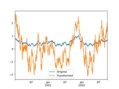
Suppose we wish to standardize the data within each group:
In [129]:index=pd.date_range("10/1/1999",periods=1100)In [130]:ts=pd.Series(np.random.normal(0.5,2,1100),index)In [131]:ts=ts.rolling(window=100,min_periods=100).mean().dropna()In [132]:ts.head()Out[132]:2000-01-08 0.7793332000-01-09 0.7788522000-01-10 0.7864762000-01-11 0.7827972000-01-12 0.798110Freq: D, dtype: float64In [133]:ts.tail()Out[133]:2002-09-30 0.6602942002-10-01 0.6310952002-10-02 0.6736012002-10-03 0.7092132002-10-04 0.719369Freq: D, dtype: float64In [134]:transformed=ts.groupby(lambdax:x.year).transform( .....:lambdax:(x-x.mean())/x.std() .....:) .....:
We would expect the result to now have mean 0 and standard deviation 1 withineach group (up to floating-point error), which we can easily check:
# Original DataIn [135]:grouped=ts.groupby(lambdax:x.year)In [136]:grouped.mean()Out[136]:2000 0.4424412001 0.5262462002 0.459365dtype: float64In [137]:grouped.std()Out[137]:2000 0.1317522001 0.2109452002 0.128753dtype: float64# Transformed DataIn [138]:grouped_trans=transformed.groupby(lambdax:x.year)In [139]:grouped_trans.mean()Out[139]:2000 -4.870756e-162001 -1.545187e-162002 4.136282e-16dtype: float64In [140]:grouped_trans.std()Out[140]:2000 1.02001 1.02002 1.0dtype: float64
We can also visually compare the original and transformed data sets.
In [141]:compare=pd.DataFrame({"Original":ts,"Transformed":transformed})In [142]:compare.plot()Out[142]:<Axes: >
Transformation functions that have lower dimension outputs are broadcast tomatch the shape of the input array.
In [143]:ts.groupby(lambdax:x.year).transform(lambdax:x.max()-x.min())Out[143]:2000-01-08 0.6238932000-01-09 0.6238932000-01-10 0.6238932000-01-11 0.6238932000-01-12 0.623893 ...2002-09-30 0.5582752002-10-01 0.5582752002-10-02 0.5582752002-10-03 0.5582752002-10-04 0.558275Freq: D, Length: 1001, dtype: float64
Another common data transform is to replace missing data with the group mean.
In [144]:cols=["A","B","C"]In [145]:values=np.random.randn(1000,3)In [146]:values[np.random.randint(0,1000,100),0]=np.nanIn [147]:values[np.random.randint(0,1000,50),1]=np.nanIn [148]:values[np.random.randint(0,1000,200),2]=np.nanIn [149]:data_df=pd.DataFrame(values,columns=cols)In [150]:data_dfOut[150]: A B C0 1.539708 -1.166480 0.5330261 1.302092 -0.505754 NaN2 -0.371983 1.104803 -0.6515203 -1.309622 1.118697 -1.1616574 -1.924296 0.396437 0.812436.. ... ... ...995 -0.093110 0.683847 -0.774753996 -0.185043 1.438572 NaN997 -0.394469 -0.642343 0.011374998 -1.174126 1.857148 NaN999 0.234564 0.517098 0.393534[1000 rows x 3 columns]In [151]:countries=np.array(["US","UK","GR","JP"])In [152]:key=countries[np.random.randint(0,4,1000)]In [153]:grouped=data_df.groupby(key)# Non-NA count in each groupIn [154]:grouped.count()Out[154]: A B CGR 209 217 189JP 240 255 217UK 216 231 193US 239 250 217In [155]:transformed=grouped.transform(lambdax:x.fillna(x.mean()))
We can verify that the group means have not changed in the transformed data,and that the transformed data contains no NAs.
In [156]:grouped_trans=transformed.groupby(key)In [157]:grouped.mean()# original group meansOut[157]: A B CGR -0.098371 -0.015420 0.068053JP 0.069025 0.023100 -0.077324UK 0.034069 -0.052580 -0.116525US 0.058664 -0.020399 0.028603In [158]:grouped_trans.mean()# transformation did not change group meansOut[158]: A B CGR -0.098371 -0.015420 0.068053JP 0.069025 0.023100 -0.077324UK 0.034069 -0.052580 -0.116525US 0.058664 -0.020399 0.028603In [159]:grouped.count()# original has some missing data pointsOut[159]: A B CGR 209 217 189JP 240 255 217UK 216 231 193US 239 250 217In [160]:grouped_trans.count()# counts after transformationOut[160]: A B CGR 228 228 228JP 267 267 267UK 247 247 247US 258 258 258In [161]:grouped_trans.size()# Verify non-NA count equals group sizeOut[161]:GR 228JP 267UK 247US 258dtype: int64
As mentioned in the note above, each of the examples in this section can be computedmore efficiently using built-in methods. In the code below, the inefficient wayusing a UDF is commented out and the faster alternative appears below.
# result = ts.groupby(lambda x: x.year).transform(# lambda x: (x - x.mean()) / x.std()# )In [162]:grouped=ts.groupby(lambdax:x.year)In [163]:result=(ts-grouped.transform("mean"))/grouped.transform("std")# result = ts.groupby(lambda x: x.year).transform(lambda x: x.max() - x.min())In [164]:grouped=ts.groupby(lambdax:x.year)In [165]:result=grouped.transform("max")-grouped.transform("min")# grouped = data_df.groupby(key)# result = grouped.transform(lambda x: x.fillna(x.mean()))In [166]:grouped=data_df.groupby(key)In [167]:result=data_df.fillna(grouped.transform("mean"))
Window and resample operations#
It is possible to useresample(),expanding() androlling() as methods on groupbys.
The example below will apply therolling() method on the samples ofthe column B, based on the groups of column A.
In [168]:df_re=pd.DataFrame({"A":[1]*10+[5]*10,"B":np.arange(20)})In [169]:df_reOut[169]: A B0 1 01 1 12 1 23 1 34 1 4.. .. ..15 5 1516 5 1617 5 1718 5 1819 5 19[20 rows x 2 columns]In [170]:df_re.groupby("A").rolling(4).B.mean()Out[170]:A1 0 NaN 1 NaN 2 NaN 3 1.5 4 2.5 ...5 15 13.5 16 14.5 17 15.5 18 16.5 19 17.5Name: B, Length: 20, dtype: float64
Theexpanding() method will accumulate a given operation(sum() in the example) for all the members of each particulargroup.
In [171]:df_re.groupby("A").expanding().sum()Out[171]: BA1 0 0.0 1 1.0 2 3.0 3 6.0 4 10.0... ...5 15 75.0 16 91.0 17 108.0 18 126.0 19 145.0[20 rows x 1 columns]
Suppose you want to use theresample() method to get a dailyfrequency in each group of your dataframe, and wish to complete themissing values with theffill() method.
In [172]:df_re=pd.DataFrame( .....:{ .....:"date":pd.date_range(start="2016-01-01",periods=4,freq="W"), .....:"group":[1,1,2,2], .....:"val":[5,6,7,8], .....:} .....:).set_index("date") .....:In [173]:df_reOut[173]: group valdate2016-01-03 1 52016-01-10 1 62016-01-17 2 72016-01-24 2 8In [174]:df_re.groupby("group").resample("1D",include_groups=False).ffill()Out[174]: valgroup date1 2016-01-03 5 2016-01-04 5 2016-01-05 5 2016-01-06 5 2016-01-07 5... ...2 2016-01-20 7 2016-01-21 7 2016-01-22 7 2016-01-23 7 2016-01-24 8[16 rows x 1 columns]
Filtration#
A filtration is a GroupBy operation that subsets the original grouping object. Itmay either filter out entire groups, part of groups, or both. Filtrations returna filtered version of the calling object, including the grouping columns when provided.In the following example,class is included in the result.
In [175]:speedsOut[175]: class order max_speedfalcon bird Falconiformes 389.0parrot bird Psittaciformes 24.0lion mammal Carnivora 80.2monkey mammal Primates NaNleopard mammal Carnivora 58.0In [176]:speeds.groupby("class").nth(1)Out[176]: class order max_speedparrot bird Psittaciformes 24.0monkey mammal Primates NaN
Note
Unlike aggregations, filtrations do not add the group keys to the index of theresult. Because of this, passingas_index=False orsort=True will notaffect these methods.
Filtrations will respect subsetting the columns of the GroupBy object.
In [177]:speeds.groupby("class")[["order","max_speed"]].nth(1)Out[177]: order max_speedparrot Psittaciformes 24.0monkey Primates NaN
Built-in filtrations#
The following methods on GroupBy act as filtrations. All these methods have anefficient, GroupBy-specific, implementation.
Method | Description |
|---|---|
Select the top row(s) of each group | |
Select the nth row(s) of each group | |
Select the bottom row(s) of each group |
Users can also use transformations along with Boolean indexing to construct complexfiltrations within groups. For example, suppose we are given groups of products andtheir volumes, and we wish to subset the data to only the largest products capturing nomore than 90% of the total volume within each group.
In [178]:product_volumes=pd.DataFrame( .....:{ .....:"group":list("xxxxyyy"), .....:"product":list("abcdefg"), .....:"volume":[10,30,20,15,40,10,20], .....:} .....:) .....:In [179]:product_volumesOut[179]: group product volume0 x a 101 x b 302 x c 203 x d 154 y e 405 y f 106 y g 20# Sort by volume to select the largest products firstIn [180]:product_volumes=product_volumes.sort_values("volume",ascending=False)In [181]:grouped=product_volumes.groupby("group")["volume"]In [182]:cumpct=grouped.cumsum()/grouped.transform("sum")In [183]:cumpctOut[183]:4 0.5714291 0.4000002 0.6666676 0.8571433 0.8666670 1.0000005 1.000000Name: volume, dtype: float64In [184]:significant_products=product_volumes[cumpct<=0.9]In [185]:significant_products.sort_values(["group","product"])Out[185]: group product volume1 x b 302 x c 203 x d 154 y e 406 y g 20
Thefilter method#
Note
Filtering by supplyingfilter with a User-Defined Function (UDF) isoften less performant than using the built-in methods on GroupBy.Consider breaking up a complex operation into a chain of operations that utilizethe built-in methods.
Thefilter method takes a User-Defined Function (UDF) that, when applied toan entire group, returns eitherTrue orFalse. The result of thefiltermethod is then the subset of groups for which the UDF returnedTrue.
Suppose we want to take only elements that belong to groups with a group sum greaterthan 2.
In [186]:sf=pd.Series([1,1,2,3,3,3])In [187]:sf.groupby(sf).filter(lambdax:x.sum()>2)Out[187]:3 34 35 3dtype: int64
Another useful operation is filtering out elements that belong to groupswith only a couple members.
In [188]:dff=pd.DataFrame({"A":np.arange(8),"B":list("aabbbbcc")})In [189]:dff.groupby("B").filter(lambdax:len(x)>2)Out[189]: A B2 2 b3 3 b4 4 b5 5 b
Alternatively, instead of dropping the offending groups, we can return alike-indexed objects where the groups that do not pass the filter are filledwith NaNs.
In [190]:dff.groupby("B").filter(lambdax:len(x)>2,dropna=False)Out[190]: A B0 NaN NaN1 NaN NaN2 2.0 b3 3.0 b4 4.0 b5 5.0 b6 NaN NaN7 NaN NaN
For DataFrames with multiple columns, filters should explicitly specify a column as the filter criterion.
In [191]:dff["C"]=np.arange(8)In [192]:dff.groupby("B").filter(lambdax:len(x["C"])>2)Out[192]: A B C2 2 b 23 3 b 34 4 b 45 5 b 5
Flexibleapply#
Some operations on the grouped data might not fit into the aggregation,transformation, or filtration categories. For these, you can use theapplyfunction.
Warning
apply has to try to infer from the result whether it should act as a reducer,transformer,or filter, depending on exactly what is passed to it. Thus thegrouped column(s) may be included in the output or not. Whileit tries to intelligently guess how to behave, it can sometimes guess wrong.
Note
All of the examples in this section can be more reliably, and more efficiently,computed using other pandas functionality.
In [193]:dfOut[193]: A B C D0 foo one -0.575247 1.3460611 bar one 0.254161 1.5117632 foo two -1.143704 1.6270813 bar three 0.215897 -0.9905824 foo two 1.193555 -0.4416525 bar two -0.077118 1.2115266 foo one -0.408530 0.2685207 foo three -0.862495 0.024580In [194]:grouped=df.groupby("A")# could also just call .describe()In [195]:grouped["C"].apply(lambdax:x.describe())Out[195]:Abar count 3.000000 mean 0.130980 std 0.181231 min -0.077118 25% 0.069390 ...foo min -1.143704 25% -0.862495 50% -0.575247 75% -0.408530 max 1.193555Name: C, Length: 16, dtype: float64
The dimension of the returned result can also change:
In [196]:grouped=df.groupby('A')['C']In [197]:deff(group): .....:returnpd.DataFrame({'original':group, .....:'demeaned':group-group.mean()}) .....:In [198]:grouped.apply(f)Out[198]: original demeanedAbar 1 0.254161 0.123181 3 0.215897 0.084917 5 -0.077118 -0.208098foo 0 -0.575247 -0.215962 2 -1.143704 -0.784420 4 1.193555 1.552839 6 -0.408530 -0.049245 7 -0.862495 -0.503211
apply on a Series can operate on a returned value from the applied functionthat is itself a series, and possibly upcast the result to a DataFrame:
In [199]:deff(x): .....:returnpd.Series([x,x**2],index=["x","x^2"]) .....:In [200]:s=pd.Series(np.random.rand(5))In [201]:sOut[201]:0 0.5828981 0.0983522 0.0014383 0.0094204 0.815826dtype: float64In [202]:s.apply(f)Out[202]: x x^20 0.582898 0.3397701 0.098352 0.0096732 0.001438 0.0000023 0.009420 0.0000894 0.815826 0.665572
Similar toThe aggregate() method, the resulting dtype will reflect that of theapply function. If the results from different groups have different dtypes, thena common dtype will be determined in the same way asDataFrame construction.
Control grouped column(s) placement withgroup_keys#
To control whether the grouped column(s) are included in the indices, you can usethe argumentgroup_keys which defaults toTrue. Compare
In [203]:df.groupby("A",group_keys=True).apply(lambdax:x,include_groups=False)Out[203]: B C DAbar 1 one 0.254161 1.511763 3 three 0.215897 -0.990582 5 two -0.077118 1.211526foo 0 one -0.575247 1.346061 2 two -1.143704 1.627081 4 two 1.193555 -0.441652 6 one -0.408530 0.268520 7 three -0.862495 0.024580
with
In [204]:df.groupby("A",group_keys=False).apply(lambdax:x,include_groups=False)Out[204]: B C D0 one -0.575247 1.3460611 one 0.254161 1.5117632 two -1.143704 1.6270813 three 0.215897 -0.9905824 two 1.193555 -0.4416525 two -0.077118 1.2115266 one -0.408530 0.2685207 three -0.862495 0.024580
Numba Accelerated Routines#
Added in version 1.1.
IfNumba is installed as an optional dependency, thetransform andaggregate methods supportengine='numba' andengine_kwargs arguments.Seeenhancing performance with Numba for general usage of the argumentsand performance considerations.
The function signature must start withvalues,indexexactly as the data belonging to each groupwill be passed intovalues, and the group index will be passed intoindex.
Warning
When usingengine='numba', there will be no “fall back” behavior internally. The groupdata and group index will be passed as NumPy arrays to the JITed user defined function, and noalternative execution attempts will be tried.
Other useful features#
Exclusion of non-numeric columns#
Again consider the example DataFrame we’ve been looking at:
In [205]:dfOut[205]: A B C D0 foo one -0.575247 1.3460611 bar one 0.254161 1.5117632 foo two -1.143704 1.6270813 bar three 0.215897 -0.9905824 foo two 1.193555 -0.4416525 bar two -0.077118 1.2115266 foo one -0.408530 0.2685207 foo three -0.862495 0.024580
Suppose we wish to compute the standard deviation grouped by theAcolumn. There is a slight problem, namely that we don’t care about the data incolumnB because it is not numeric. You can avoid non-numeric columns byspecifyingnumeric_only=True:
In [206]:df.groupby("A").std(numeric_only=True)Out[206]: C DAbar 0.181231 1.366330foo 0.912265 0.884785
Note thatdf.groupby('A').colname.std(). is more efficient thandf.groupby('A').std().colname. So if the result of an aggregation functionis only needed over one column (herecolname), it may be filteredbefore applying the aggregation function.
In [207]:fromdecimalimportDecimalIn [208]:df_dec=pd.DataFrame( .....:{ .....:"id":[1,2,1,2], .....:"int_column":[1,2,3,4], .....:"dec_column":[ .....:Decimal("0.50"), .....:Decimal("0.15"), .....:Decimal("0.25"), .....:Decimal("0.40"), .....:], .....:} .....:) .....:In [209]:df_dec.groupby(["id"])[["dec_column"]].sum()Out[209]: dec_columnid1 0.752 0.55
Handling of (un)observed Categorical values#
When using aCategorical grouper (as a single grouper, or as part of multiple groupers), theobserved keywordcontrols whether to return a cartesian product of all possible groupers values (observed=False) or only thosethat are observed groupers (observed=True).
Show all values:
In [210]:pd.Series([1,1,1]).groupby( .....:pd.Categorical(["a","a","a"],categories=["a","b"]),observed=False .....:).count() .....:Out[210]:a 3b 0dtype: int64
Show only the observed values:
In [211]:pd.Series([1,1,1]).groupby( .....:pd.Categorical(["a","a","a"],categories=["a","b"]),observed=True .....:).count() .....:Out[211]:a 3dtype: int64
The returned dtype of the grouped willalways includeall of the categories that were grouped.
In [212]:s=( .....:pd.Series([1,1,1]) .....:.groupby(pd.Categorical(["a","a","a"],categories=["a","b"]),observed=True) .....:.count() .....:) .....:In [213]:s.index.dtypeOut[213]:CategoricalDtype(categories=['a', 'b'], ordered=False, categories_dtype=object)
NA group handling#
ByNA, we are referring to anyNA values, includingNA,NaN,NaT, andNone. If there are anyNA values in thegrouping key, by default these will be excluded. In other words, any“NA group” will be dropped. You can include NA groups by specifyingdropna=False.
In [214]:df=pd.DataFrame({"key":[1.0,1.0,np.nan,2.0,np.nan],"A":[1,2,3,4,5]})In [215]:dfOut[215]: key A0 1.0 11 1.0 22 NaN 33 2.0 44 NaN 5In [216]:df.groupby("key",dropna=True).sum()Out[216]: Akey1.0 32.0 4In [217]:df.groupby("key",dropna=False).sum()Out[217]: Akey1.0 32.0 4NaN 8
Grouping with ordered factors#
Categorical variables represented as instances of pandas’sCategorical classcan be used as group keys. If so, the order of the levels will be preserved. Whenobserved=False andsort=False, any unobserved categories will be at theend of the result in order.
In [218]:days=pd.Categorical( .....:values=["Wed","Mon","Thu","Mon","Wed","Sat"], .....:categories=["Mon","Tue","Wed","Thu","Fri","Sat","Sun"], .....:) .....:In [219]:data=pd.DataFrame( .....:{ .....:"day":days, .....:"workers":[3,4,1,4,2,2], .....:} .....:) .....:In [220]:dataOut[220]: day workers0 Wed 31 Mon 42 Thu 13 Mon 44 Wed 25 Sat 2In [221]:data.groupby("day",observed=False,sort=True).sum()Out[221]: workersdayMon 8Tue 0Wed 5Thu 1Fri 0Sat 2Sun 0In [222]:data.groupby("day",observed=False,sort=False).sum()Out[222]: workersdayWed 5Mon 8Thu 1Sat 2Tue 0Fri 0Sun 0
Grouping with a grouper specification#
You may need to specify a bit more data to properly group. You canuse thepd.Grouper to provide this local control.
In [223]:importdatetimeIn [224]:df=pd.DataFrame( .....:{ .....:"Branch":"A A A A A A A B".split(), .....:"Buyer":"Carl Mark Carl Carl Joe Joe Joe Carl".split(), .....:"Quantity":[1,3,5,1,8,1,9,3], .....:"Date":[ .....:datetime.datetime(2013,1,1,13,0), .....:datetime.datetime(2013,1,1,13,5), .....:datetime.datetime(2013,10,1,20,0), .....:datetime.datetime(2013,10,2,10,0), .....:datetime.datetime(2013,10,1,20,0), .....:datetime.datetime(2013,10,2,10,0), .....:datetime.datetime(2013,12,2,12,0), .....:datetime.datetime(2013,12,2,14,0), .....:], .....:} .....:) .....:In [225]:dfOut[225]: Branch Buyer Quantity Date0 A Carl 1 2013-01-01 13:00:001 A Mark 3 2013-01-01 13:05:002 A Carl 5 2013-10-01 20:00:003 A Carl 1 2013-10-02 10:00:004 A Joe 8 2013-10-01 20:00:005 A Joe 1 2013-10-02 10:00:006 A Joe 9 2013-12-02 12:00:007 B Carl 3 2013-12-02 14:00:00
Groupby a specific column with the desired frequency. This is like resampling.
In [226]:df.groupby([pd.Grouper(freq="1ME",key="Date"),"Buyer"])[["Quantity"]].sum()Out[226]: QuantityDate Buyer2013-01-31 Carl 1 Mark 32013-10-31 Carl 6 Joe 92013-12-31 Carl 3 Joe 9
Whenfreq is specified, the object returned bypd.Grouper will be aninstance ofpandas.api.typing.TimeGrouper. When there is a column and indexwith the same name, you can usekey to group by the column andlevelto group by the index.
In [227]:df=df.set_index("Date")In [228]:df["Date"]=df.index+pd.offsets.MonthEnd(2)In [229]:df.groupby([pd.Grouper(freq="6ME",key="Date"),"Buyer"])[["Quantity"]].sum()Out[229]: QuantityDate Buyer2013-02-28 Carl 1 Mark 32014-02-28 Carl 9 Joe 18In [230]:df.groupby([pd.Grouper(freq="6ME",level="Date"),"Buyer"])[["Quantity"]].sum()Out[230]: QuantityDate Buyer2013-01-31 Carl 1 Mark 32014-01-31 Carl 9 Joe 18
Taking the first rows of each group#
Just like for a DataFrame or Series you can call head and tail on a groupby:
In [231]:df=pd.DataFrame([[1,2],[1,4],[5,6]],columns=["A","B"])In [232]:dfOut[232]: A B0 1 21 1 42 5 6In [233]:g=df.groupby("A")In [234]:g.head(1)Out[234]: A B0 1 22 5 6In [235]:g.tail(1)Out[235]: A B1 1 42 5 6
This shows the first or last n rows from each group.
Taking the nth row of each group#
To select the nth item from each group, useDataFrameGroupBy.nth() orSeriesGroupBy.nth(). Arguments supplied can be any integer, lists of integers,slices, or lists of slices; see below for examples. When the nth element of a groupdoes not exist an error isnot raised; instead no corresponding rows are returned.
In general this operation acts as a filtration. In certain cases it will also returnone row per group, making it also a reduction. However because in general it canreturn zero or multiple rows per group, pandas treats it as a filtration in all cases.
In [236]:df=pd.DataFrame([[1,np.nan],[1,4],[5,6]],columns=["A","B"])In [237]:g=df.groupby("A")In [238]:g.nth(0)Out[238]: A B0 1 NaN2 5 6.0In [239]:g.nth(-1)Out[239]: A B1 1 4.02 5 6.0In [240]:g.nth(1)Out[240]: A B1 1 4.0
If the nth element of a group does not exist, then no corresponding row is includedin the result. In particular, if the specifiedn is larger than any group, theresult will be an empty DataFrame.
In [241]:g.nth(5)Out[241]:Empty DataFrameColumns: [A, B]Index: []
If you want to select the nth not-null item, use thedropna kwarg. For a DataFrame this should be either'any' or'all' just like you would pass to dropna:
# nth(0) is the same as g.first()In [242]:g.nth(0,dropna="any")Out[242]: A B1 1 4.02 5 6.0In [243]:g.first()Out[243]: BA1 4.05 6.0# nth(-1) is the same as g.last()In [244]:g.nth(-1,dropna="any")Out[244]: A B1 1 4.02 5 6.0In [245]:g.last()Out[245]: BA1 4.05 6.0In [246]:g.B.nth(0,dropna="all")Out[246]:1 4.02 6.0Name: B, dtype: float64
You can also select multiple rows from each group by specifying multiple nth values as a list of ints.
In [247]:business_dates=pd.date_range(start="4/1/2014",end="6/30/2014",freq="B")In [248]:df=pd.DataFrame(1,index=business_dates,columns=["a","b"])# get the first, 4th, and last date index for each monthIn [249]:df.groupby([df.index.year,df.index.month]).nth([0,3,-1])Out[249]: a b2014-04-01 1 12014-04-04 1 12014-04-30 1 12014-05-01 1 12014-05-06 1 12014-05-30 1 12014-06-02 1 12014-06-05 1 12014-06-30 1 1
You may also use slices or lists of slices.
In [250]:df.groupby([df.index.year,df.index.month]).nth[1:]Out[250]: a b2014-04-02 1 12014-04-03 1 12014-04-04 1 12014-04-07 1 12014-04-08 1 1... .. ..2014-06-24 1 12014-06-25 1 12014-06-26 1 12014-06-27 1 12014-06-30 1 1[62 rows x 2 columns]In [251]:df.groupby([df.index.year,df.index.month]).nth[1:,:-1]Out[251]: a b2014-04-01 1 12014-04-02 1 12014-04-03 1 12014-04-04 1 12014-04-07 1 1... .. ..2014-06-24 1 12014-06-25 1 12014-06-26 1 12014-06-27 1 12014-06-30 1 1[65 rows x 2 columns]
Enumerate group items#
To see the order in which each row appears within its group, use thecumcount method:
In [252]:dfg=pd.DataFrame(list("aaabba"),columns=["A"])In [253]:dfgOut[253]: A0 a1 a2 a3 b4 b5 aIn [254]:dfg.groupby("A").cumcount()Out[254]:0 01 12 23 04 15 3dtype: int64In [255]:dfg.groupby("A").cumcount(ascending=False)Out[255]:0 31 22 13 14 05 0dtype: int64
Enumerate groups#
To see the ordering of the groups (as opposed to the order of rowswithin a group given bycumcount) you can useDataFrameGroupBy.ngroup().
Note that the numbers given to the groups match the order in which thegroups would be seen when iterating over the groupby object, not theorder they are first observed.
In [256]:dfg=pd.DataFrame(list("aaabba"),columns=["A"])In [257]:dfgOut[257]: A0 a1 a2 a3 b4 b5 aIn [258]:dfg.groupby("A").ngroup()Out[258]:0 01 02 03 14 15 0dtype: int64In [259]:dfg.groupby("A").ngroup(ascending=False)Out[259]:0 11 12 13 04 05 1dtype: int64
Plotting#
Groupby also works with some plotting methods. In this case, suppose wesuspect that the values in column 1 are 3 times higher on average in group “B”.
In [260]:np.random.seed(1234)In [261]:df=pd.DataFrame(np.random.randn(50,2))In [262]:df["g"]=np.random.choice(["A","B"],size=50)In [263]:df.loc[df["g"]=="B",1]+=3
We can easily visualize this with a boxplot:
In [264]:df.groupby("g").boxplot()Out[264]:A Axes(0.1,0.15;0.363636x0.75)B Axes(0.536364,0.15;0.363636x0.75)dtype: object
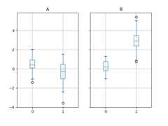
The result of callingboxplot is a dictionary whose keys are the valuesof our grouping columng (“A” and “B”). The values of the resulting dictionarycan be controlled by thereturn_type keyword ofboxplot.See thevisualization documentation for more.
Warning
For historical reasons,df.groupby("g").boxplot() is not equivalenttodf.boxplot(by="g"). Seehere foran explanation.
Piping function calls#
Similar to the functionality provided byDataFrame andSeries, functionsthat takeGroupBy objects can be chained together using apipe method toallow for a cleaner, more readable syntax. To read about.pipe in general terms,seehere.
Combining.groupby and.pipe is often useful when you need to reuseGroupBy objects.
As an example, imagine having a DataFrame with columns for stores, products,revenue and quantity sold. We’d like to do a groupwise calculation ofprices(i.e. revenue/quantity) per store and per product. We could do this in amulti-step operation, but expressing it in terms of piping can make thecode more readable. First we set the data:
In [265]:n=1000In [266]:df=pd.DataFrame( .....:{ .....:"Store":np.random.choice(["Store_1","Store_2"],n), .....:"Product":np.random.choice(["Product_1","Product_2"],n), .....:"Revenue":(np.random.random(n)*50+10).round(2), .....:"Quantity":np.random.randint(1,10,size=n), .....:} .....:) .....:In [267]:df.head(2)Out[267]: Store Product Revenue Quantity0 Store_2 Product_1 26.12 11 Store_2 Product_1 28.86 1
We now find the prices per store/product.
In [268]:( .....:df.groupby(["Store","Product"]) .....:.pipe(lambdagrp:grp.Revenue.sum()/grp.Quantity.sum()) .....:.unstack() .....:.round(2) .....:) .....:Out[268]:Product Product_1 Product_2StoreStore_1 6.82 7.05Store_2 6.30 6.64
Piping can also be expressive when you want to deliver a grouped object to somearbitrary function, for example:
In [269]:defmean(groupby): .....:returngroupby.mean() .....:In [270]:df.groupby(["Store","Product"]).pipe(mean)Out[270]: Revenue QuantityStore ProductStore_1 Product_1 34.622727 5.075758 Product_2 35.482815 5.029630Store_2 Product_1 32.972837 5.237589 Product_2 34.684360 5.224000
Heremean takes a GroupBy object and finds the mean of the Revenue and Quantitycolumns respectively for each Store-Product combination. Themean function canbe any function that takes in a GroupBy object; the.pipe will pass the GroupByobject as a parameter into the function you specify.
Examples#
Multi-column factorization#
By usingDataFrameGroupBy.ngroup(), we can extractinformation about the groups in a way similar tofactorize() (as describedfurther in thereshaping API) but which appliesnaturally to multiple columns of mixed type and differentsources. This can be useful as an intermediate categorical-like stepin processing, when the relationships between the group rows are moreimportant than their content, or as input to an algorithm which onlyaccepts the integer encoding. (For more information about support inpandas for full categorical data, see theCategoricalintroduction and theAPI documentation.)
In [271]:dfg=pd.DataFrame({"A":[1,1,2,3,2],"B":list("aaaba")})In [272]:dfgOut[272]: A B0 1 a1 1 a2 2 a3 3 b4 2 aIn [273]:dfg.groupby(["A","B"]).ngroup()Out[273]:0 01 02 13 24 1dtype: int64In [274]:dfg.groupby(["A",[0,0,0,1,1]]).ngroup()Out[274]:0 01 02 13 34 2dtype: int64
Groupby by indexer to ‘resample’ data#
Resampling produces new hypothetical samples (resamples) from already existing observed data or from a model that generates data. These new samples are similar to the pre-existing samples.
In order for resample to work on indices that are non-datetimelike, the following procedure can be utilized.
In the following examples,df.index // 5 returns an integer array which is used to determine what gets selected for the groupby operation.
Note
The example below shows how we can downsample by consolidation of samples into fewer ones.Here by usingdf.index // 5, we are aggregating the samples in bins. By applyingstd()function, we aggregate the information contained in many samples into a small subset of valueswhich is their standard deviation thereby reducing the number of samples.
In [275]:df=pd.DataFrame(np.random.randn(10,2))In [276]:dfOut[276]: 0 10 -0.793893 0.3211531 0.342250 1.6189062 -0.975807 1.9182013 -0.810847 -1.4059194 -1.977759 0.4616595 0.730057 -1.3169386 -0.751328 0.5282907 -0.257759 -1.0810098 0.505895 -1.7019489 -1.006349 0.020208In [277]:df.index//5Out[277]:Index([0, 0, 0, 0, 0, 1, 1, 1, 1, 1], dtype='int64')In [278]:df.groupby(df.index//5).std()Out[278]: 0 10 0.823647 1.3129121 0.760109 0.942941
Returning a Series to propagate names#
Group DataFrame columns, compute a set of metrics and return a named Series.The Series name is used as the name for the column index. This is especiallyuseful in conjunction with reshaping operations such as stacking, in which thecolumn index name will be used as the name of the inserted column:
In [279]:df=pd.DataFrame( .....:{ .....:"a":[0,0,0,0,1,1,1,1,2,2,2,2], .....:"b":[0,0,1,1,0,0,1,1,0,0,1,1], .....:"c":[1,0,1,0,1,0,1,0,1,0,1,0], .....:"d":[0,0,0,1,0,0,0,1,0,0,0,1], .....:} .....:) .....:In [280]:defcompute_metrics(x): .....:result={"b_sum":x["b"].sum(),"c_mean":x["c"].mean()} .....:returnpd.Series(result,name="metrics") .....:In [281]:result=df.groupby("a").apply(compute_metrics,include_groups=False)In [282]:resultOut[282]:metrics b_sum c_meana0 2.0 0.51 2.0 0.52 2.0 0.5In [283]:result.stack(future_stack=True)Out[283]:a metrics0 b_sum 2.0 c_mean 0.51 b_sum 2.0 c_mean 0.52 b_sum 2.0 c_mean 0.5dtype: float64