10 minutes to pandas#
This is a short introduction to pandas, geared mainly for new users.You can see more complex recipes in theCookbook.
Customarily, we import as follows:
In [1]:importnumpyasnpIn [2]:importpandasaspd
Basic data structures in pandas#
Pandas provides two types of classes for handling data:
Object creation#
See theIntro to data structures section.
Creating aSeries by passing a list of values, letting pandas createa defaultRangeIndex.
In [3]:s=pd.Series([1,3,5,np.nan,6,8])In [4]:sOut[4]:0 1.01 3.02 5.03 NaN4 6.05 8.0dtype: float64
Creating aDataFrame by passing a NumPy array with a datetime index usingdate_range()and labeled columns:
In [5]:dates=pd.date_range("20130101",periods=6)In [6]:datesOut[6]:DatetimeIndex(['2013-01-01', '2013-01-02', '2013-01-03', '2013-01-04', '2013-01-05', '2013-01-06'], dtype='datetime64[ns]', freq='D')In [7]:df=pd.DataFrame(np.random.randn(6,4),index=dates,columns=list("ABCD"))In [8]:dfOut[8]: A B C D2013-01-01 0.469112 -0.282863 -1.509059 -1.1356322013-01-02 1.212112 -0.173215 0.119209 -1.0442362013-01-03 -0.861849 -2.104569 -0.494929 1.0718042013-01-04 0.721555 -0.706771 -1.039575 0.2718602013-01-05 -0.424972 0.567020 0.276232 -1.0874012013-01-06 -0.673690 0.113648 -1.478427 0.524988
Creating aDataFrame by passing a dictionary of objects where the keys are the columnlabels and the values are the column values.
In [9]:df2=pd.DataFrame( ...:{ ...:"A":1.0, ...:"B":pd.Timestamp("20130102"), ...:"C":pd.Series(1,index=list(range(4)),dtype="float32"), ...:"D":np.array([3]*4,dtype="int32"), ...:"E":pd.Categorical(["test","train","test","train"]), ...:"F":"foo", ...:} ...:) ...:In [10]:df2Out[10]: A B C D E F0 1.0 2013-01-02 1.0 3 test foo1 1.0 2013-01-02 1.0 3 train foo2 1.0 2013-01-02 1.0 3 test foo3 1.0 2013-01-02 1.0 3 train foo
The columns of the resultingDataFrame have differentdtypes:
In [11]:df2.dtypesOut[11]:A float64B datetime64[s]C float32D int32E categoryF objectdtype: object
If you’re using IPython, tab completion for column names (as well as publicattributes) is automatically enabled. Here’s a subset of the attributes thatwill be completed:
In [12]:df2.<TAB># noqa: E225, E999df2.A df2.booldf2.abs df2.boxplotdf2.add df2.Cdf2.add_prefix df2.clipdf2.add_suffix df2.columnsdf2.align df2.copydf2.all df2.countdf2.any df2.combinedf2.append df2.Ddf2.apply df2.describedf2.applymap df2.diffdf2.B df2.duplicated
As you can see, the columnsA,B,C, andD are automaticallytab completed.E andF are there as well; the rest of the attributes have beentruncated for brevity.
Viewing data#
See theEssentially basics functionality section.
UseDataFrame.head() andDataFrame.tail() to view the top and bottom rows of the framerespectively:
In [13]:df.head()Out[13]: A B C D2013-01-01 0.469112 -0.282863 -1.509059 -1.1356322013-01-02 1.212112 -0.173215 0.119209 -1.0442362013-01-03 -0.861849 -2.104569 -0.494929 1.0718042013-01-04 0.721555 -0.706771 -1.039575 0.2718602013-01-05 -0.424972 0.567020 0.276232 -1.087401In [14]:df.tail(3)Out[14]: A B C D2013-01-04 0.721555 -0.706771 -1.039575 0.2718602013-01-05 -0.424972 0.567020 0.276232 -1.0874012013-01-06 -0.673690 0.113648 -1.478427 0.524988
Display theDataFrame.index orDataFrame.columns:
In [15]:df.indexOut[15]:DatetimeIndex(['2013-01-01', '2013-01-02', '2013-01-03', '2013-01-04', '2013-01-05', '2013-01-06'], dtype='datetime64[ns]', freq='D')In [16]:df.columnsOut[16]:Index(['A', 'B', 'C', 'D'], dtype='object')
Return a NumPy representation of the underlying data withDataFrame.to_numpy()without the index or column labels:
In [17]:df.to_numpy()Out[17]:array([[ 0.4691, -0.2829, -1.5091, -1.1356], [ 1.2121, -0.1732, 0.1192, -1.0442], [-0.8618, -2.1046, -0.4949, 1.0718], [ 0.7216, -0.7068, -1.0396, 0.2719], [-0.425 , 0.567 , 0.2762, -1.0874], [-0.6737, 0.1136, -1.4784, 0.525 ]])
Note
NumPy arrays have one dtype for the entire array while pandas DataFrameshave one dtype per column. When you callDataFrame.to_numpy(), pandas willfind the NumPy dtype that can holdall of the dtypes in the DataFrame.If the common data type isobject,DataFrame.to_numpy() will requirecopying data.
In [18]:df2.dtypesOut[18]:A float64B datetime64[s]C float32D int32E categoryF objectdtype: objectIn [19]:df2.to_numpy()Out[19]:array([[1.0, Timestamp('2013-01-02 00:00:00'), 1.0, 3, 'test', 'foo'], [1.0, Timestamp('2013-01-02 00:00:00'), 1.0, 3, 'train', 'foo'], [1.0, Timestamp('2013-01-02 00:00:00'), 1.0, 3, 'test', 'foo'], [1.0, Timestamp('2013-01-02 00:00:00'), 1.0, 3, 'train', 'foo']], dtype=object)
describe() shows a quick statistic summary of your data:
In [20]:df.describe()Out[20]: A B C Dcount 6.000000 6.000000 6.000000 6.000000mean 0.073711 -0.431125 -0.687758 -0.233103std 0.843157 0.922818 0.779887 0.973118min -0.861849 -2.104569 -1.509059 -1.13563225% -0.611510 -0.600794 -1.368714 -1.07661050% 0.022070 -0.228039 -0.767252 -0.38618875% 0.658444 0.041933 -0.034326 0.461706max 1.212112 0.567020 0.276232 1.071804
Transposing your data:
In [21]:df.TOut[21]: 2013-01-01 2013-01-02 2013-01-03 2013-01-04 2013-01-05 2013-01-06A 0.469112 1.212112 -0.861849 0.721555 -0.424972 -0.673690B -0.282863 -0.173215 -2.104569 -0.706771 0.567020 0.113648C -1.509059 0.119209 -0.494929 -1.039575 0.276232 -1.478427D -1.135632 -1.044236 1.071804 0.271860 -1.087401 0.524988
DataFrame.sort_index() sorts by an axis:
In [22]:df.sort_index(axis=1,ascending=False)Out[22]: D C B A2013-01-01 -1.135632 -1.509059 -0.282863 0.4691122013-01-02 -1.044236 0.119209 -0.173215 1.2121122013-01-03 1.071804 -0.494929 -2.104569 -0.8618492013-01-04 0.271860 -1.039575 -0.706771 0.7215552013-01-05 -1.087401 0.276232 0.567020 -0.4249722013-01-06 0.524988 -1.478427 0.113648 -0.673690
DataFrame.sort_values() sorts by values:
In [23]:df.sort_values(by="B")Out[23]: A B C D2013-01-03 -0.861849 -2.104569 -0.494929 1.0718042013-01-04 0.721555 -0.706771 -1.039575 0.2718602013-01-01 0.469112 -0.282863 -1.509059 -1.1356322013-01-02 1.212112 -0.173215 0.119209 -1.0442362013-01-06 -0.673690 0.113648 -1.478427 0.5249882013-01-05 -0.424972 0.567020 0.276232 -1.087401
Selection#
Note
While standard Python / NumPy expressions for selecting and setting areintuitive and come in handy for interactive work, for production code, werecommend the optimized pandas data access methods,DataFrame.at(),DataFrame.iat(),DataFrame.loc() andDataFrame.iloc().
See the indexing documentationIndexing and Selecting Data andMultiIndex / Advanced Indexing.
Getitem ([])#
For aDataFrame, passing a single label selects a columns andyields aSeries equivalent todf.A:
In [24]:df["A"]Out[24]:2013-01-01 0.4691122013-01-02 1.2121122013-01-03 -0.8618492013-01-04 0.7215552013-01-05 -0.4249722013-01-06 -0.673690Freq: D, Name: A, dtype: float64
For aDataFrame, passing a slice: selects matching rows:
In [25]:df[0:3]Out[25]: A B C D2013-01-01 0.469112 -0.282863 -1.509059 -1.1356322013-01-02 1.212112 -0.173215 0.119209 -1.0442362013-01-03 -0.861849 -2.104569 -0.494929 1.071804In [26]:df["20130102":"20130104"]Out[26]: A B C D2013-01-02 1.212112 -0.173215 0.119209 -1.0442362013-01-03 -0.861849 -2.104569 -0.494929 1.0718042013-01-04 0.721555 -0.706771 -1.039575 0.271860
Selection by label#
See more inSelection by Label usingDataFrame.loc() orDataFrame.at().
Selecting a row matching a label:
In [27]:df.loc[dates[0]]Out[27]:A 0.469112B -0.282863C -1.509059D -1.135632Name: 2013-01-01 00:00:00, dtype: float64
Selecting all rows (:) with a select column labels:
In [28]:df.loc[:,["A","B"]]Out[28]: A B2013-01-01 0.469112 -0.2828632013-01-02 1.212112 -0.1732152013-01-03 -0.861849 -2.1045692013-01-04 0.721555 -0.7067712013-01-05 -0.424972 0.5670202013-01-06 -0.673690 0.113648
For label slicing, both endpoints areincluded:
In [29]:df.loc["20130102":"20130104",["A","B"]]Out[29]: A B2013-01-02 1.212112 -0.1732152013-01-03 -0.861849 -2.1045692013-01-04 0.721555 -0.706771
Selecting a single row and column label returns a scalar:
In [30]:df.loc[dates[0],"A"]Out[30]:0.4691122999071863
For getting fast access to a scalar (equivalent to the prior method):
In [31]:df.at[dates[0],"A"]Out[31]:0.4691122999071863
Selection by position#
See more inSelection by Position usingDataFrame.iloc() orDataFrame.iat().
Select via the position of the passed integers:
In [32]:df.iloc[3]Out[32]:A 0.721555B -0.706771C -1.039575D 0.271860Name: 2013-01-04 00:00:00, dtype: float64
Integer slices acts similar to NumPy/Python:
In [33]:df.iloc[3:5,0:2]Out[33]: A B2013-01-04 0.721555 -0.7067712013-01-05 -0.424972 0.567020
Lists of integer position locations:
In [34]:df.iloc[[1,2,4],[0,2]]Out[34]: A C2013-01-02 1.212112 0.1192092013-01-03 -0.861849 -0.4949292013-01-05 -0.424972 0.276232
For slicing rows explicitly:
In [35]:df.iloc[1:3,:]Out[35]: A B C D2013-01-02 1.212112 -0.173215 0.119209 -1.0442362013-01-03 -0.861849 -2.104569 -0.494929 1.071804
For slicing columns explicitly:
In [36]:df.iloc[:,1:3]Out[36]: B C2013-01-01 -0.282863 -1.5090592013-01-02 -0.173215 0.1192092013-01-03 -2.104569 -0.4949292013-01-04 -0.706771 -1.0395752013-01-05 0.567020 0.2762322013-01-06 0.113648 -1.478427
For getting a value explicitly:
In [37]:df.iloc[1,1]Out[37]:-0.17321464905330858
For getting fast access to a scalar (equivalent to the prior method):
In [38]:df.iat[1,1]Out[38]:-0.17321464905330858
Boolean indexing#
Select rows wheredf.A is greater than0.
In [39]:df[df["A"]>0]Out[39]: A B C D2013-01-01 0.469112 -0.282863 -1.509059 -1.1356322013-01-02 1.212112 -0.173215 0.119209 -1.0442362013-01-04 0.721555 -0.706771 -1.039575 0.271860
Selecting values from aDataFrame where a boolean condition is met:
In [40]:df[df>0]Out[40]: A B C D2013-01-01 0.469112 NaN NaN NaN2013-01-02 1.212112 NaN 0.119209 NaN2013-01-03 NaN NaN NaN 1.0718042013-01-04 0.721555 NaN NaN 0.2718602013-01-05 NaN 0.567020 0.276232 NaN2013-01-06 NaN 0.113648 NaN 0.524988
Usingisin() method for filtering:
In [41]:df2=df.copy()In [42]:df2["E"]=["one","one","two","three","four","three"]In [43]:df2Out[43]: A B C D E2013-01-01 0.469112 -0.282863 -1.509059 -1.135632 one2013-01-02 1.212112 -0.173215 0.119209 -1.044236 one2013-01-03 -0.861849 -2.104569 -0.494929 1.071804 two2013-01-04 0.721555 -0.706771 -1.039575 0.271860 three2013-01-05 -0.424972 0.567020 0.276232 -1.087401 four2013-01-06 -0.673690 0.113648 -1.478427 0.524988 threeIn [44]:df2[df2["E"].isin(["two","four"])]Out[44]: A B C D E2013-01-03 -0.861849 -2.104569 -0.494929 1.071804 two2013-01-05 -0.424972 0.567020 0.276232 -1.087401 four
Setting#
Setting a new column automatically aligns the data by the indexes:
In [45]:s1=pd.Series([1,2,3,4,5,6],index=pd.date_range("20130102",periods=6))In [46]:s1Out[46]:2013-01-02 12013-01-03 22013-01-04 32013-01-05 42013-01-06 52013-01-07 6Freq: D, dtype: int64In [47]:df["F"]=s1
Setting values by label:
In [48]:df.at[dates[0],"A"]=0
Setting values by position:
In [49]:df.iat[0,1]=0
Setting by assigning with a NumPy array:
In [50]:df.loc[:,"D"]=np.array([5]*len(df))
The result of the prior setting operations:
In [51]:dfOut[51]: A B C D F2013-01-01 0.000000 0.000000 -1.509059 5.0 NaN2013-01-02 1.212112 -0.173215 0.119209 5.0 1.02013-01-03 -0.861849 -2.104569 -0.494929 5.0 2.02013-01-04 0.721555 -0.706771 -1.039575 5.0 3.02013-01-05 -0.424972 0.567020 0.276232 5.0 4.02013-01-06 -0.673690 0.113648 -1.478427 5.0 5.0
Awhere operation with setting:
In [52]:df2=df.copy()In [53]:df2[df2>0]=-df2In [54]:df2Out[54]: A B C D F2013-01-01 0.000000 0.000000 -1.509059 -5.0 NaN2013-01-02 -1.212112 -0.173215 -0.119209 -5.0 -1.02013-01-03 -0.861849 -2.104569 -0.494929 -5.0 -2.02013-01-04 -0.721555 -0.706771 -1.039575 -5.0 -3.02013-01-05 -0.424972 -0.567020 -0.276232 -5.0 -4.02013-01-06 -0.673690 -0.113648 -1.478427 -5.0 -5.0
Missing data#
For NumPy data types,np.nan represents missing data. It is bydefault not included in computations. See theMissing Data section.
Reindexing allows you to change/add/delete the index on a specified axis. Thisreturns a copy of the data:
In [55]:df1=df.reindex(index=dates[0:4],columns=list(df.columns)+["E"])In [56]:df1.loc[dates[0]:dates[1],"E"]=1In [57]:df1Out[57]: A B C D F E2013-01-01 0.000000 0.000000 -1.509059 5.0 NaN 1.02013-01-02 1.212112 -0.173215 0.119209 5.0 1.0 1.02013-01-03 -0.861849 -2.104569 -0.494929 5.0 2.0 NaN2013-01-04 0.721555 -0.706771 -1.039575 5.0 3.0 NaN
DataFrame.dropna() drops any rows that have missing data:
In [58]:df1.dropna(how="any")Out[58]: A B C D F E2013-01-02 1.212112 -0.173215 0.119209 5.0 1.0 1.0
DataFrame.fillna() fills missing data:
In [59]:df1.fillna(value=5)Out[59]: A B C D F E2013-01-01 0.000000 0.000000 -1.509059 5.0 5.0 1.02013-01-02 1.212112 -0.173215 0.119209 5.0 1.0 1.02013-01-03 -0.861849 -2.104569 -0.494929 5.0 2.0 5.02013-01-04 0.721555 -0.706771 -1.039575 5.0 3.0 5.0
isna() gets the boolean mask where values arenan:
In [60]:pd.isna(df1)Out[60]: A B C D F E2013-01-01 False False False False True False2013-01-02 False False False False False False2013-01-03 False False False False False True2013-01-04 False False False False False True
Operations#
See theBasic section on Binary Ops.
Stats#
Operations in generalexclude missing data.
Calculate the mean value for each column:
In [61]:df.mean()Out[61]:A -0.004474B -0.383981C -0.687758D 5.000000F 3.000000dtype: float64
Calculate the mean value for each row:
In [62]:df.mean(axis=1)Out[62]:2013-01-01 0.8727352013-01-02 1.4316212013-01-03 0.7077312013-01-04 1.3950422013-01-05 1.8836562013-01-06 1.592306Freq: D, dtype: float64
Operating with anotherSeries orDataFrame with a different index or columnwill align the result with the union of the index or column labels. In addition, pandasautomatically broadcasts along the specified dimension and will fill unaligned labels withnp.nan.
In [63]:s=pd.Series([1,3,5,np.nan,6,8],index=dates).shift(2)In [64]:sOut[64]:2013-01-01 NaN2013-01-02 NaN2013-01-03 1.02013-01-04 3.02013-01-05 5.02013-01-06 NaNFreq: D, dtype: float64In [65]:df.sub(s,axis="index")Out[65]: A B C D F2013-01-01 NaN NaN NaN NaN NaN2013-01-02 NaN NaN NaN NaN NaN2013-01-03 -1.861849 -3.104569 -1.494929 4.0 1.02013-01-04 -2.278445 -3.706771 -4.039575 2.0 0.02013-01-05 -5.424972 -4.432980 -4.723768 0.0 -1.02013-01-06 NaN NaN NaN NaN NaN
User defined functions#
DataFrame.agg() andDataFrame.transform() applies a user defined functionthat reduces or broadcasts its result respectively.
In [66]:df.agg(lambdax:np.mean(x)*5.6)Out[66]:A -0.025054B -2.150294C -3.851445D 28.000000F 16.800000dtype: float64In [67]:df.transform(lambdax:x*101.2)Out[67]: A B C D F2013-01-01 0.000000 0.000000 -152.716721 506.0 NaN2013-01-02 122.665737 -17.529322 12.063922 506.0 101.22013-01-03 -87.219115 -212.982405 -50.086843 506.0 202.42013-01-04 73.021382 -71.525239 -105.204988 506.0 303.62013-01-05 -43.007200 57.382459 27.954680 506.0 404.82013-01-06 -68.177398 11.501219 -149.616767 506.0 506.0
Value Counts#
See more atHistogramming and Discretization.
In [68]:s=pd.Series(np.random.randint(0,7,size=10))In [69]:sOut[69]:0 41 22 13 24 65 46 47 68 49 4dtype: int64In [70]:s.value_counts()Out[70]:4 52 26 21 1Name: count, dtype: int64
String Methods#
Series is equipped with a set of string processing methods in thestrattribute that make it easy to operate on each element of the array, as in thecode snippet below. See more atVectorized String Methods.
In [71]:s=pd.Series(["A","B","C","Aaba","Baca",np.nan,"CABA","dog","cat"])In [72]:s.str.lower()Out[72]:0 a1 b2 c3 aaba4 baca5 NaN6 caba7 dog8 catdtype: object
Merge#
Concat#
pandas provides various facilities for easily combining togetherSeries andDataFrame objects with various kinds of set logic for the indexesand relational algebra functionality in the case of join / merge-typeoperations.
See theMerging section.
Concatenating pandas objects together row-wise withconcat():
In [73]:df=pd.DataFrame(np.random.randn(10,4))In [74]:dfOut[74]: 0 1 2 30 -0.548702 1.467327 -1.015962 -0.4830751 1.637550 -1.217659 -0.291519 -1.7455052 -0.263952 0.991460 -0.919069 0.2660463 -0.709661 1.669052 1.037882 -1.7057754 -0.919854 -0.042379 1.247642 -0.0099205 0.290213 0.495767 0.362949 1.5481066 -1.131345 -0.089329 0.337863 -0.9458677 -0.932132 1.956030 0.017587 -0.0166928 -0.575247 0.254161 -1.143704 0.2158979 1.193555 -0.077118 -0.408530 -0.862495# break it into piecesIn [75]:pieces=[df[:3],df[3:7],df[7:]]In [76]:pd.concat(pieces)Out[76]: 0 1 2 30 -0.548702 1.467327 -1.015962 -0.4830751 1.637550 -1.217659 -0.291519 -1.7455052 -0.263952 0.991460 -0.919069 0.2660463 -0.709661 1.669052 1.037882 -1.7057754 -0.919854 -0.042379 1.247642 -0.0099205 0.290213 0.495767 0.362949 1.5481066 -1.131345 -0.089329 0.337863 -0.9458677 -0.932132 1.956030 0.017587 -0.0166928 -0.575247 0.254161 -1.143704 0.2158979 1.193555 -0.077118 -0.408530 -0.862495
Join#
merge() enables SQL style join types along specific columns. See theDatabase style joining section.
In [77]:left=pd.DataFrame({"key":["foo","foo"],"lval":[1,2]})In [78]:right=pd.DataFrame({"key":["foo","foo"],"rval":[4,5]})In [79]:leftOut[79]: key lval0 foo 11 foo 2In [80]:rightOut[80]: key rval0 foo 41 foo 5In [81]:pd.merge(left,right,on="key")Out[81]: key lval rval0 foo 1 41 foo 1 52 foo 2 43 foo 2 5
merge() on unique keys:
In [82]:left=pd.DataFrame({"key":["foo","bar"],"lval":[1,2]})In [83]:right=pd.DataFrame({"key":["foo","bar"],"rval":[4,5]})In [84]:leftOut[84]: key lval0 foo 11 bar 2In [85]:rightOut[85]: key rval0 foo 41 bar 5In [86]:pd.merge(left,right,on="key")Out[86]: key lval rval0 foo 1 41 bar 2 5
Grouping#
By “group by” we are referring to a process involving one or more of thefollowing steps:
Splitting the data into groups based on some criteria
Applying a function to each group independently
Combining the results into a data structure
See theGrouping section.
In [87]:df=pd.DataFrame( ....:{ ....:"A":["foo","bar","foo","bar","foo","bar","foo","foo"], ....:"B":["one","one","two","three","two","two","one","three"], ....:"C":np.random.randn(8), ....:"D":np.random.randn(8), ....:} ....:) ....:In [88]:dfOut[88]: A B C D0 foo one 1.346061 -1.5775851 bar one 1.511763 0.3968232 foo two 1.627081 -0.1053813 bar three -0.990582 -0.5325324 foo two -0.441652 1.4537495 bar two 1.211526 1.2088436 foo one 0.268520 -0.0809527 foo three 0.024580 -0.264610
Grouping by a column label, selecting column labels, and then applying theDataFrameGroupBy.sum() function to the resultinggroups:
In [89]:df.groupby("A")[["C","D"]].sum()Out[89]: C DAbar 1.732707 1.073134foo 2.824590 -0.574779
Grouping by multiple columns label formsMultiIndex.
In [90]:df.groupby(["A","B"]).sum()Out[90]: C DA Bbar one 1.511763 0.396823 three -0.990582 -0.532532 two 1.211526 1.208843foo one 1.614581 -1.658537 three 0.024580 -0.264610 two 1.185429 1.348368
Reshaping#
See the sections onHierarchical Indexing andReshaping.
Stack#
In [91]:arrays=[ ....:["bar","bar","baz","baz","foo","foo","qux","qux"], ....:["one","two","one","two","one","two","one","two"], ....:] ....:In [92]:index=pd.MultiIndex.from_arrays(arrays,names=["first","second"])In [93]:df=pd.DataFrame(np.random.randn(8,2),index=index,columns=["A","B"])In [94]:df2=df[:4]In [95]:df2Out[95]: A Bfirst secondbar one -0.727965 -0.589346 two 0.339969 -0.693205baz one -0.339355 0.593616 two 0.884345 1.591431
Thestack() method “compresses” a level in the DataFrame’scolumns:
In [96]:stacked=df2.stack(future_stack=True)In [97]:stackedOut[97]:first secondbar one A -0.727965 B -0.589346 two A 0.339969 B -0.693205baz one A -0.339355 B 0.593616 two A 0.884345 B 1.591431dtype: float64
With a “stacked” DataFrame or Series (having aMultiIndex as theindex), the inverse operation ofstack() isunstack(), which by default unstacks thelast level:
In [98]:stacked.unstack()Out[98]: A Bfirst secondbar one -0.727965 -0.589346 two 0.339969 -0.693205baz one -0.339355 0.593616 two 0.884345 1.591431In [99]:stacked.unstack(1)Out[99]:second one twofirstbar A -0.727965 0.339969 B -0.589346 -0.693205baz A -0.339355 0.884345 B 0.593616 1.591431In [100]:stacked.unstack(0)Out[100]:first bar bazsecondone A -0.727965 -0.339355 B -0.589346 0.593616two A 0.339969 0.884345 B -0.693205 1.591431
Pivot tables#
See the section onPivot Tables.
In [101]:df=pd.DataFrame( .....:{ .....:"A":["one","one","two","three"]*3, .....:"B":["A","B","C"]*4, .....:"C":["foo","foo","foo","bar","bar","bar"]*2, .....:"D":np.random.randn(12), .....:"E":np.random.randn(12), .....:} .....:) .....:In [102]:dfOut[102]: A B C D E0 one A foo -1.202872 0.0476091 one B foo -1.814470 -0.1364732 two C foo 1.018601 -0.5617573 three A bar -0.595447 -1.6230334 one B bar 1.395433 0.0293995 one C bar -0.392670 -0.5421086 two A foo 0.007207 0.2826967 three B foo 1.928123 -0.0873028 one C foo -0.055224 -1.5751709 one A bar 2.395985 1.77120810 two B bar 1.552825 0.81648211 three C bar 0.166599 1.100230
pivot_table() pivots aDataFrame specifying thevalues,index andcolumns
In [103]:pd.pivot_table(df,values="D",index=["A","B"],columns=["C"])Out[103]:C bar fooA Bone A 2.395985 -1.202872 B 1.395433 -1.814470 C -0.392670 -0.055224three A -0.595447 NaN B NaN 1.928123 C 0.166599 NaNtwo A NaN 0.007207 B 1.552825 NaN C NaN 1.018601
Time series#
pandas has simple, powerful, and efficient functionality for performingresampling operations during frequency conversion (e.g., converting secondlydata into 5-minutely data). This is extremely common in, but not limited to,financial applications. See theTime Series section.
In [104]:rng=pd.date_range("1/1/2012",periods=100,freq="s")In [105]:ts=pd.Series(np.random.randint(0,500,len(rng)),index=rng)In [106]:ts.resample("5Min").sum()Out[106]:2012-01-01 24182Freq: 5min, dtype: int64
Series.tz_localize() localizes a time series to a time zone:
In [107]:rng=pd.date_range("3/6/2012 00:00",periods=5,freq="D")In [108]:ts=pd.Series(np.random.randn(len(rng)),rng)In [109]:tsOut[109]:2012-03-06 1.8577042012-03-07 -1.1935452012-03-08 0.6775102012-03-09 -0.1539312012-03-10 0.520091Freq: D, dtype: float64In [110]:ts_utc=ts.tz_localize("UTC")In [111]:ts_utcOut[111]:2012-03-06 00:00:00+00:00 1.8577042012-03-07 00:00:00+00:00 -1.1935452012-03-08 00:00:00+00:00 0.6775102012-03-09 00:00:00+00:00 -0.1539312012-03-10 00:00:00+00:00 0.520091Freq: D, dtype: float64
Series.tz_convert() converts a timezones aware time series to another time zone:
In [112]:ts_utc.tz_convert("US/Eastern")Out[112]:2012-03-05 19:00:00-05:00 1.8577042012-03-06 19:00:00-05:00 -1.1935452012-03-07 19:00:00-05:00 0.6775102012-03-08 19:00:00-05:00 -0.1539312012-03-09 19:00:00-05:00 0.520091Freq: D, dtype: float64
Adding a non-fixed duration (BusinessDay) to a time series:
In [113]:rngOut[113]:DatetimeIndex(['2012-03-06', '2012-03-07', '2012-03-08', '2012-03-09', '2012-03-10'], dtype='datetime64[ns]', freq='D')In [114]:rng+pd.offsets.BusinessDay(5)Out[114]:DatetimeIndex(['2012-03-13', '2012-03-14', '2012-03-15', '2012-03-16', '2012-03-16'], dtype='datetime64[ns]', freq=None)
Categoricals#
pandas can include categorical data in aDataFrame. For full docs, see thecategorical introduction and theAPI documentation.
In [115]:df=pd.DataFrame( .....:{"id":[1,2,3,4,5,6],"raw_grade":["a","b","b","a","a","e"]} .....:) .....:
Converting the raw grades to a categorical data type:
In [116]:df["grade"]=df["raw_grade"].astype("category")In [117]:df["grade"]Out[117]:0 a1 b2 b3 a4 a5 eName: grade, dtype: categoryCategories (3, object): ['a', 'b', 'e']
Rename the categories to more meaningful names:
In [118]:new_categories=["very good","good","very bad"]In [119]:df["grade"]=df["grade"].cat.rename_categories(new_categories)
Reorder the categories and simultaneously add the missing categories (methods underSeries.cat() return a newSeries by default):
In [120]:df["grade"]=df["grade"].cat.set_categories( .....:["very bad","bad","medium","good","very good"] .....:) .....:In [121]:df["grade"]Out[121]:0 very good1 good2 good3 very good4 very good5 very badName: grade, dtype: categoryCategories (5, object): ['very bad', 'bad', 'medium', 'good', 'very good']
Sorting is per order in the categories, not lexical order:
In [122]:df.sort_values(by="grade")Out[122]: id raw_grade grade5 6 e very bad1 2 b good2 3 b good0 1 a very good3 4 a very good4 5 a very good
Grouping by a categorical column withobserved=False also shows empty categories:
In [123]:df.groupby("grade",observed=False).size()Out[123]:gradevery bad 1bad 0medium 0good 2very good 3dtype: int64
Plotting#
See thePlotting docs.
We use the standard convention for referencing the matplotlib API:
In [124]:importmatplotlib.pyplotaspltIn [125]:plt.close("all")
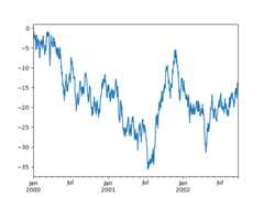
Theplt.close method is used toclose a figure window:
In [126]:ts=pd.Series(np.random.randn(1000),index=pd.date_range("1/1/2000",periods=1000))In [127]:ts=ts.cumsum()In [128]:ts.plot();
Note
When using Jupyter, the plot will appear usingplot(). Otherwise usematplotlib.pyplot.show to show it ormatplotlib.pyplot.savefig to write it to a file.
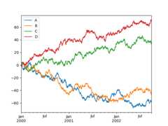
plot() plots all columns:
In [129]:df=pd.DataFrame( .....:np.random.randn(1000,4),index=ts.index,columns=["A","B","C","D"] .....:) .....:In [130]:df=df.cumsum()In [131]:plt.figure();In [132]:df.plot();In [133]:plt.legend(loc='best');
Importing and exporting data#
See theIO Tools section.
CSV#
Writing to a csv file: usingDataFrame.to_csv()
In [134]:df=pd.DataFrame(np.random.randint(0,5,(10,5)))In [135]:df.to_csv("foo.csv")
Reading from a csv file: usingread_csv()
In [136]:pd.read_csv("foo.csv")Out[136]: Unnamed: 0 0 1 2 3 40 0 4 3 1 1 21 1 1 0 2 3 22 2 1 4 2 1 23 3 0 4 0 2 24 4 4 2 2 3 45 5 4 0 4 3 16 6 2 1 2 0 37 7 4 0 4 4 48 8 4 4 1 0 19 9 0 4 3 0 3
Parquet#
Writing to a Parquet file:
In [137]:df.to_parquet("foo.parquet")
Reading from a Parquet file Store usingread_parquet():
In [138]:pd.read_parquet("foo.parquet")Out[138]: 0 1 2 3 40 4 3 1 1 21 1 0 2 3 22 1 4 2 1 23 0 4 0 2 24 4 2 2 3 45 4 0 4 3 16 2 1 2 0 37 4 0 4 4 48 4 4 1 0 19 0 4 3 0 3
Excel#
Reading and writing toExcel.
Writing to an excel file usingDataFrame.to_excel():
In [139]:df.to_excel("foo.xlsx",sheet_name="Sheet1")
Reading from an excel file usingread_excel():
In [140]:pd.read_excel("foo.xlsx","Sheet1",index_col=None,na_values=["NA"])Out[140]: Unnamed: 0 0 1 2 3 40 0 4 3 1 1 21 1 1 0 2 3 22 2 1 4 2 1 23 3 0 4 0 2 24 4 4 2 2 3 45 5 4 0 4 3 16 6 2 1 2 0 37 7 4 0 4 4 48 8 4 4 1 0 19 9 0 4 3 0 3
Gotchas#
If you are attempting to perform a boolean operation on aSeries orDataFrameyou might see an exception like:
In [141]:ifpd.Series([False,True,False]): .....:print("I was true") .....:---------------------------------------------------------------------------ValueErrorTraceback (most recent call last)<ipython-input-141-b27eb9c1dfc0> in?()---->1ifpd.Series([False,True,False]):2print("I was true")~/work/pandas/pandas/pandas/core/generic.py in?(self)1575@final1576def__nonzero__(self)->NoReturn:->1577raiseValueError(1578f"The truth value of a{type(self).__name__} is ambiguous. "1579"Use a.empty, a.bool(), a.item(), a.any() or a.all()."1580)ValueError: The truth value of a Series is ambiguous. Use a.empty, a.bool(), a.item(), a.any() or a.all().
SeeComparisons andGotchas for an explanation and what to do.