Radio Materials
A radio material defines how an object scatters incident radio waves.It implements all necessary components to simulate the interaction betweenradio waves and objects composed of specific materials.
The base classRadioMaterialBase provides an interfacefor implementing arbitrary radio materials and can be used to implementedcustom materials, as detailed in theDeveloper Guide.
TheRadioMaterial class implements the model described in thePrimer on Electromagnetics, and supports specular and diffusereflection as well as refraction. The details of this model are provided thereafter.
Similarly to scene objects (SceneObject), all radiomaterials are uniquely identified by their name.For example, specifying that a scene object named“wall” is made of thematerial named“itu-brick” is done as follows:
obj=scene.get("wall")# obj is a SceneObjectobj.radio_material="itu-brick"# "wall" is made of "itu-brick"
Radio materials provided with Sionna
The classRadioMaterial implements the model described in thePrimer on Electromagnetics. Following this model, a radio material consists of thereal-valued relative permittivity\(\varepsilon_r\), the conductivity\(\sigma\),and the relative permeability\(\mu_r\).For more details, see(7),(8),(9).These quantities can possibly depend on the frequency of the incident radiowave. Note that this model only allows non-magnetic materials with\(\mu_r=1\).
A radio material has also a thickness\(d\) associated with it which impacts the computation ofthe reflected and refracted fields (see(35)). For example, a wallis modeled in Sionna RT as a planar surface whose radio material describes thedesired thickness.
Additionally, aRadioMaterial can have an effective roughness (ER)associated with it, leading to diffuse reflections (see, e.g.,[Degli-Esposti11]).The ER model requires a scattering coefficient\(S\in[0,1]\)(39),a cross-polarization discrimination coefficient\(K_x\)(41), as well as a scattering pattern\(f_\text{s}(\hat{\mathbf{k}}_\text{i}, \hat{\mathbf{k}}_\text{s})\)(42)–(44), such as theLambertianPattern orDirectivePattern. The meaning ofthese parameters is explained inScattering.
Sionna provides theITU models of several materials whose propertiesare automatically updated according to the configuredfrequency.
Through theITURadioMaterial class, Sionna provides the models of all of the materialsdefined in the ITU-R P.2040-3 recommendation[ITU_R_2040_3]. These models are based on curve fitting tomeasurement results and assume non-ionized and non-magnetic materials(\(\mu_r = 1\)).Frequency dependence is modeled by
where\(f_{\text{GHz}}\) is the frequency in GHz, and the constants\(a\),\(b\),\(c\), and\(d\) characterize the material.The table below provides their values which are used in Sionna(from[ITU_R_2040_3]).Note that the relative permittivity\(\varepsilon_r\) andconductivity\(\sigma\) of all materials are updated automatically whenthe frequency is set through the scene’s propertyfrequency.Moreover, by default, the scattering coefficient,\(S\), of these materials is set to0, leading to no diffuse reflection.
Material type | Real part of relative permittivity | Conductivity [S/m] | Frequency range (GHz) | ||
a | b | c | d | ||
vacuum | 1 | 0 | 0 | 0 | 0.001 – 100 |
concrete | 5.24 | 0 | 0.0462 | 0.7822 | 1 – 100 |
brick | 3.91 | 0 | 0.0238 | 0.16 | 1 – 40 |
plasterboard | 2.73 | 0 | 0.0085 | 0.9395 | 1 – 100 |
wood | 1.99 | 0 | 0.0047 | 1.0718 | 0.001 – 100 |
glass | 6.31 | 0 | 0.0036 | 1.3394 | 0.1 – 100 |
5.79 | 0 | 0.0004 | 1.658 | 220 – 450 | |
ceiling_board | 1.48 | 0 | 0.0011 | 1.0750 | 1 – 100 |
1.52 | 0 | 0.0029 | 1.029 | 220 – 450 | |
chipboard | 2.58 | 0 | 0.0217 | 0.7800 | 1 – 100 |
plywood | 2.71 | 0 | 0.33 | 0 | 1 – 40 |
marble | 7.074 | 0 | 0.0055 | 0.9262 | 1 – 60 |
floorboard | 3.66 | 0 | 0.0044 | 1.3515 | 50 – 100 |
metal | 1 | 0 | \(10^7\) | 0 | 1 – 100 |
very_dry_ground | 3 | 0 | 0.00015 | 2.52 | 1 – 10 |
medium_dry_ground | 15 | -0.1 | 0.035 | 1.63 | 1 – 10 |
wet_ground | 30 | -0.4 | 0.15 | 1.30 | 1 – 10 |
- classsionna.rt.RadioMaterialBase(props)[source]
Base class to implement a radio material
This is an abstract class that cannot be instantiated, and serves asinterface for defining radio materials.
A radio material defines how an object scatters incident radio waves.
- Parameters:
props (
mitsuba.Properties) – Property container storing the parameters required to build the material
- propertycolor
Get/set the the RGB (red, green, blue) color for theradio material as displayed in the previewer and renderer.Each RGB component must have a value within the range\(\in [0,1]\).
- Type:
Tuple[float,float,float]
- eval(ctx,si,wo,active=True)[source]
Evaluates the radio material
This function evaluates the Jones matrix of the radio material for the scattereddirection
woand for the interaction type stored insi.prim_index.The following assumptions are made on the inputs:
si.wiis the direction of propagation of the incident wave in the world framesi.sh_frameis the frame such that thesh_frame.nis the normal to the intersected surface in the world coordinate systemsi.dn_dustores the real part of the S and P components of the incident electric field represented in the implicit world frame (first and second components ofsi.dn_du)si.dn_dvstores the imaginary part of the S and P components of the incident electric field represented in the implicit world frame (first and second components ofsi.dn_dv)si.dp_dustores the solid angle of the ray tube (first component ofsi.dn_du)si.prim_indexstores the interaction type to evaluate
- Parameters:
ctx (
mitsuba.BSDFContext) – A context data structure used to specify which interaction types are enabledsi (
mitsuba.SurfaceInteraction3f) – Surface interaction data structure describing the underlying surface positionwo (
mitsuba.Vector3f) – Direction of propagation of the scattered wave in the world frameactive (
bool|drjit.cuda.ad.Bool) – Mask to specify active rays
- Return type:
mitsuba.Spectrum- Returns:
Jones matrix as a\(4 \times 4\) real-valued matrix
- propertyname
(read-only) Name of the radio material
- Type:
str
- pdf(ctx,si,wo,active=True)[source]
Evaluates the probability of the sampled interaction type and direction of scattered ray
This function evaluates the probability density of the radio material for the scattereddirection
woand for the interaction type stored insi.prim_index.The following assumptions are made on the inputs:
si.wiis the direction of propagation of the incident wave in the world framesi.sh_frameis the frame such that thesh_frame.nis the normal to the intersected surface in the world coordinate systemsi.dn_dustores the real part of the S and P components of the incident electric field represented in the implicit world frame (first and second components ofsi.dn_du)si.dn_dvstores the imaginary part of the S and P components of the incident electric field represented in the implicit world frame (first and second components ofsi.dn_dv)si.dp_dustores the solid angle of the ray tube (first component ofsi.dn_du)si.prim_indexstores the interaction type to evaluate
- Parameters:
ctx (
mitsuba.BSDFContext) – A context data structure used to specify which interaction types are enabledsi (
mitsuba.SurfaceInteraction3f) – Surface interaction data structure describing the underlying surface positionwo (
mitsuba.Vector3f) – Direction of propagation of the scattered wave in the world frameactive (
bool|drjit.cuda.ad.Bool) – Mask to specify active rays
- Return type:
drjit.cuda.ad.Float- Returns:
Probability density value
- sample(ctx,si,sample1,sample2,active=True)[source]
Samples the radio material
This function samples an interaction type (e.g., specular reflection,diffuse reflection or refraction) and direction of propagation for thescattered ray, and returns the corresponding radio material sample and Jones matrix.The returned radio material sample stores the sampled type of interaction and sampled directionof propagation of the scattered ray.
The following assumptions are made on the inputs:
ctx.componentis a binary mask that specifies the types of interaction enabled. Booleans can be obtained from this mask as follows:
specular_reflection_enabled=(ctx.component&InteractionType.SPECULAR)>0diffuse_reflection_enabled=(ctx.component&InteractionType.DIFFUSE)>0transmission_enabled=(ctx.component&InteractionType.TRANSMISSION)>0
si.wiis the direction of propagation of the incident wave in the world framesi.sh_frameis the frame such that thesh_frame.nis the normal to the intersected surface in the world coordinate systemsi.dn_dustores the real part of the S and P components of the incident electric field represented in the implicit world frame (first and second components ofsi.dn_du)si.dn_dvstores the imaginary part of the S and P components of the incident electric field represented in the implicit world frame (first and second components ofsi.dn_dv)si.dp_dustores the solid angle of the ray tube (first component ofsi.dn_du)
The outputs are set as follows:
bs.wois the direction of propagation of the sampled scattered ray in the world framejones_matis the Jones matrix describing the transformation incurred to the incident wave in the implicit world frame
- Parameters:
ctx (
mitsuba.BSDFContext) – A context data structure used to specify which interaction types are enabledsi (
mitsuba.SurfaceInteraction3f) – Surface interaction data structure describing the underlying surface positionsample1 (
drjit.cuda.ad.Float) – A uniformly distributed sample on\([0,1]\) used to sample the type of interactionsample2 (
mitsuba.Point2f) – A uniformly distributed sample on\([0,1]^2\) used to sample the direction of the reflected wave in the case of diffuse reflectionactive (
bool|drjit.cuda.ad.Bool) – Mask to specify active rays
- Return type:
typing.Tuple[mitsuba.BSDFSample3f,mitsuba.Spectrum]- Returns:
Radio material sample and Jones matrix as a\(4 \times 4\) real-valued matrix
- propertyscene
Get/set the scene used by the radio material.Note that the scene can only be set once.
- Type:
- traverse(callback)[source]
Traverse the attributes and objects of this instance
Implementing this function is required for Mitsuba to traverse a scene graph,including materials, and determine the differentiable parameters.
- Parameters:
callback (
mitsuba.TraversalCallback) – Object used to traverse the scene graph
- classsionna.rt.RadioMaterial(name=None,thickness=0.1,relative_permittivity=1.0,conductivity=0.0,scattering_coefficient=0.0,xpd_coefficient=0.0,scattering_pattern='lambertian',frequency_update_callback=None,color=None,props=None,**kwargs)[source]
Class implementing the radio material model described in thePrimer on Electromagnetics
This class implements
RadioMaterialBase.A radio material is defined by its relative permittivity\(\varepsilon_r\) and conductivity\(\sigma\) (see(9)), itsthickness\(d\) (see(36)),as well as optional parameters related to diffuse reflection (seeScattering), such as thescattering coefficient\(S\), cross-polarization discriminationcoefficient\(K_x\), and scattering pattern\(f_\text{s}(\hat{\mathbf{k}}_\text{i}, \hat{\mathbf{k}}_\text{s})\).
We assume non-ionized and non-magnetic materials, and therefore thepermeability\(\mu\) of the material is assumed to be equalto the permeability of vacuum i.e.,\(\mu_r=1.0\).
Reflection and refraction coefficients are computed assuming that theintersected surface models a slab with the specified
thickness(see(35)). The computed coefficients therefore account forthe multiple internal reflections inside the slab, meaning that thisclass should be used when objects like walls are modeled as single flatsurfaces. The figure below illustrates this model, where\(E_i\) is theincident electric field,\(E_r\) is the reflected field and\(E_t\) isthe transmitted field. The Jones matrices,\(\mathbf{R}(d)\) and\(\mathbf{T}(d)\), represent the effects of reflection and transmission,respectively, and depend on the slab thickness,\(d\).
For frequency-dependent materials, it is possible tospecify a callback function
frequency_update_callbackthat computesthe material properties\((\varepsilon_r, \sigma)\) from thefrequency. If a callback function is specified, the material propertiescannot be set and the values specified at instantiation are ignored.In addition to the following inputs, additional keyword arguments can beprovided that will be passed to the scattering pattern as keywordarguments.
- Parameters:
name (
typing.Optional[str]) – Unique name of the material. Ignored ifpropsis provided.thickness (
float|drjit.cuda.ad.Float) – Thickness of the material [m]. Ignored ifpropsis provided.relative_permittivity (
float|drjit.cuda.ad.Float) – Relative permittivity of the material. Must be larger or equal to 1. Ignored iffrequency_update_callbackorpropsis provided.conductivity (
float|drjit.cuda.ad.Float) – Conductivity of the material [S/m]. Must be non-negative. Ignored iffrequency_update_callbackorpropsis provided.scattering_coefficient (
float|drjit.cuda.ad.Float) – Scattering coefficient\(S\in[0,1]\) as defined in(39). Ignored ifpropsis provided.xpd_coefficient (
float|drjit.cuda.ad.Float) – Cross-polarization discrimination coefficient\(K_x\in[0,1]\) as defined in(41). Only relevant ifscattering_coefficientis not equal to zero. Ignored ifpropsis provided.scattering_pattern (
str) – Name of a registered scattering pattern fordiffuse reflections(“lambertian” | “backscattering” | “directive”).Only relevant ifscattering_coefficientis not equal to zero. Ignored ifpropsis provided.frequency_update_callback (
typing.Optional[typing.Callable[[drjit.cuda.ad.Float],typing.Tuple[drjit.cuda.ad.Float,drjit.cuda.ad.Float]]]) – Callable used to update the material parameters when the frequency is set. This callable must take as input the frequency [Hz] and must return the material properties as a tuple:(relative_permittivity,conductivity). If set toNone, then material properties are constant and equal to the value set at instantiation or using the corresponding setters.color (
typing.Optional[typing.Tuple[float,float,float]]) – RGB (red, green, blue) color for the radio material as displayed in the previewer and renderer. Each RGB component must have a value within the range\([0,1]\). If set toNone, then a random color is used.props (
typing.Optional[mitsuba.Properties]) – Mitsuba container storing the material properties, and usedwhen loading a scene to initialize the radio material.
- Keyword Arguments:
**kwargs (
Any) – Depending on the chosen scattering antenna pattern, other keyword argumentsmust be provided.See theDeveloper Guide formore details.
- propertyfrequency_update_callback
Get/set the frequency update callback
- Type:
Callable[[mi.Float], [mi.Float,mi.Float]]
- propertyscattering_pattern
Get/set the scattering pattern
- Type:
- propertythickness
Get/set the material thickness [m]
- Type:
mi.Float

- classsionna.rt.ITURadioMaterial(name=None,itu_type=None,thickness=None,scattering_coefficient=0.0,xpd_coefficient=0.0,scattering_pattern=None,color=None,props=None,**kwargs)[source]
Class implementing the materials defined in the ITU-R P.2040-3 recommendation[ITU_R_2040_3]
This class inherits from
RadioMaterial.The models from the ITU-R P.2040-3 recommendation are based on curve fittingto measurement results and assume non-ionized and non-magnetic materials (\(\mu_r = 1\)).Frequency dependence is modeled by
\[\begin{split}\begin{align} \varepsilon_r &= a f_{\text{GHz}}^b\\ \sigma &= c f_{\text{GHz}}^d\end{align}\end{split}\]where\(f_{\text{GHz}}\) is the frequency in GHz, and the constants\(a\),\(b\),\(c\), and\(d\) characterize the material.
Note that the relative permittivity\(\varepsilon_r\) andconductivity\(\sigma\) of all materials are updated automatically whenthe frequency is set through the scene’s property
frequency.In addition to the following inputs, additional keyword arguments can beprovided that will be passed to the scattering pattern as keywordarguments.
- Parameters:
name (
typing.Optional[str]) – Unique name of the material. Ignored ifpropsis provided.itu_type (
typing.Optional[str]) – Type the ITU material. The available materials are listed inthe corresponding table. Ignored ifpropsis provided.thickness (
typing.Union[float,drjit.cuda.ad.Float,None]) – Thickness of the material [m]. Ignored ifpropsis provided.scattering_coefficient (
float|drjit.cuda.ad.Float) – Scattering coefficient\(S\in[0,1]\) as defined in(39). Ignored ifpropsis provided.xpd_coefficient (
float|drjit.cuda.ad.Float) – Cross-polarization discrimination coefficient\(K_x\in[0,1]\) as defined in(41). Only relevant ifscattering_coefficientis not equal to zero. Ignored ifpropsis provided.scattering_pattern (
typing.Optional[typing.Callable[[mitsuba.Vector3f,mitsuba.Vector3f,...],drjit.cuda.ad.Float]]) – Scattering pattern to use for diffuse reflection. Only relevant ifscattering_coefficientis not equal to zero. Ignored ifpropsis provided. Defaults tolambertian_pattern().color (
typing.Optional[typing.Tuple[float,float,float]]) – RGB (red, green, blue) color for the radio material as displayed in the previewer and renderer. Each RGB component must have a value within the range\([0,1]\). If set toNone, then a random color is used.props (
typing.Optional[mitsuba.Properties]) – Mitsuba container storing the material properties, and used when loading a scene to initialize the radio material.
- propertyitu_type
Get the ITU type
- Type:
str
Scattering Patterns
- classsionna.rt.ScatteringPattern[source]
Abstract class implementing a scattering pattern
- abstract__call__(ki_local,ko_local)[source]
- Parameters:
ki_local (
mitsuba.Vector3f) – Direction of propagation of the incident wavein local frameko_local (
mitsuba.Vector3f) – Direction of propagation of the scattered wavein local frame
- Return type:
drjit.cuda.ad.Float- Returns:
Scattering pattern value
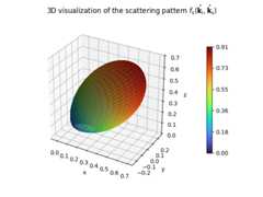
- show(k_i_local=(0.7071,0.0,-0.7071),show_directions=False)[source]
Visualizes the scattering pattern
It is assumed that the surface normal points toward thepositive z-axis.
- Parameters:
k_i_local (
mitsuba.Vector3f) – Incoming directionshow_directions (
bool) – Show incoming and specular reflectiondirections
- Return type:
tuple[matplotlib.figure.Figure,matplotlib.figure.Figure]- Returns:
3D visualization of the scattering pattern
- Returns:
Visualization of the incident plane cut throughthe scattering pattern
- classsionna.rt.LambertianPattern[source]
Lambertian scattering model from[Degli-Esposti07] as given in(42)
Example
>>>LambertianPattern().show()


- __call__(ki_local,ko_local)[source]
- Parameters:
ki_local (
mitsuba.Vector3f) – Direction of propagation of the incident wavein local frameko_local (
mitsuba.Vector3f) – Direction of propagation of the scattered wavein local frame
- Return type:
drjit.cuda.ad.Float- Returns:
Scattering pattern value
- show(k_i_local=(0.7071,0.0,-0.7071),show_directions=False)
Visualizes the scattering pattern
It is assumed that the surface normal points toward thepositive z-axis.
- Parameters:
k_i_local (
mitsuba.Vector3f) – Incoming directionshow_directions (
bool) – Show incoming and specular reflectiondirections
- Return type:
tuple[matplotlib.figure.Figure,matplotlib.figure.Figure]- Returns:
3D visualization of the scattering pattern
- Returns:
Visualization of the incident plane cut throughthe scattering pattern
- classsionna.rt.DirectivePattern(alpha_r=1)[source]
Directive scattering model from[Degli-Esposti07] as given in(43)
- Parameters:
alpha_r (
int) – Parameter related to the width of the scattering lobein the direction of the specular reflection
Example
>>>fromsionna.rtimportDirectivePattern>>>DirectivePattern(alpha_r=10).show()

- __call__(ki_local,ko_local)
- Parameters:
ki_local (
mitsuba.Vector3f) – Direction of propagation of the incident wavein local frameko_local (
mitsuba.Vector3f) – Direction of propagation of the scattered wavein local frame
- Return type:
drjit.cuda.ad.Float- Returns:
Scattering pattern value
- propertyalpha_r
Get/set\(\alpha_\text{R}\)
- Type:
int
- show(k_i_local=(0.7071,0.0,-0.7071),show_directions=False)
Visualizes the scattering pattern
It is assumed that the surface normal points toward thepositive z-axis.
- Parameters:
k_i_local (
mitsuba.Vector3f) – Incoming directionshow_directions (
bool) – Show incoming and specular reflectiondirections
- Return type:
tuple[matplotlib.figure.Figure,matplotlib.figure.Figure]- Returns:
3D visualization of the scattering pattern
- Returns:
Visualization of the incident plane cut throughthe scattering pattern
- classsionna.rt.BackscatteringPattern(alpha_r=1,alpha_i=1,lambda_=1.0)[source]
Backscattering model from[Degli-Esposti07] as given in(44)
- Parameters:
alpha_r (
int) – Parameter related to the width of the scattering lobein the direction of the specular reflectionalpha_i (
int) – Parameter related to the width of the scattering lobein the incoming directionlambda – Parameter determining the percentage of the diffuselyreflected energy in the lobe around the specular reflection
lambda_ (Float)
Example
>>>fromsionna.rtimportBackscatteringPattern>>>BackscatteringPattern(alpha_r=20,alpha_i=30,lambda_=0.7).show()


- __call__(ki_local,ko_local)[source]
- Parameters:
ki_local (
mitsuba.Vector3f) – Direction of propagation of the incident wavein local frameko_local (
mitsuba.Vector3f) – Direction of propagation of the scattered wavein local frame
- Return type:
drjit.cuda.ad.Float- Returns:
Scattering pattern value
- propertyalpha_i
Get/set\(\alpha_\text{I}\)
- Type:
int
- propertyalpha_r
Get/set\(\alpha_\text{R}\)
- Type:
int
- propertylambda_
Get/set\(\Lambda\)
- Type:
mi.float
- show(k_i_local=(0.7071,0.0,-0.7071),show_directions=False)
Visualizes the scattering pattern
It is assumed that the surface normal points toward thepositive z-axis.
- Parameters:
k_i_local (
mitsuba.Vector3f) – Incoming directionshow_directions (
bool) – Show incoming and specular reflectiondirections
- Return type:
tuple[matplotlib.figure.Figure,matplotlib.figure.Figure]- Returns:
3D visualization of the scattering pattern
- Returns:
Visualization of the incident plane cut throughthe scattering pattern
- sionna.rt.register_scattering_pattern(name,scattering_pattern_factory)[source]
Registers a new factory method for a scattering pattern
- Parameters:
name (
str) – Name of the factory methodscattering_pattern_factory (
typing.Callable[...,sionna.rt.radio_materials.scattering_pattern.ScatteringPattern]) – A factory method returning an instanceofScatteringPattern
- References:
- [Degli-Esposti11]
V. Degli-Esposti et al., “Analysis and Modeling on co- and Cross-Polarized Urban Radio Propagation for Dual-Polarized MIMO Wireless Systems”, IEEE Trans. Antennas Propag, vol. 59, no. 11, pp.4247-4256, Nov. 2011.
[ITU_R_2040_3](1,2,3)Recommendation ITU-R P.2040-3, “Effects of building materials and structures on radiowave propagation above about 100 MHz”