MIMO OFDM Transmissions over the CDL Channel Model
In this notebook, you will learn how to setup a realistic simulation of a MIMO point-to-point link between a mobile user terminal (UT) and a base station (BS). Both, uplink and downlink directions are considered. Here is a schematic diagram of the system model with all required components:
The setup includes:
5G LDPC FEC
QAM modulation
OFDM resource grid with configurabel pilot pattern
Multiple data streams
3GPP 38.901 CDL channel models and antenna patterns
ZF Precoding with perfect channel state information
LS Channel estimation with nearest-neighbor interpolation as well as perfect CSI
LMMSE MIMO equalization
You will learn how to simulate the channel in the time and frequency domains and understand when to use which option.
In particular, you will investigate:
The performance over different CDL models
The impact of imperfect CSI
Channel aging due to mobility
Inter-symbol interference due to insufficient cyclic prefix length
We will first walk through the configuration of all components of the system model, before simulating some simple transmissions in the time and frequency domain. Then, we will build a general end-to-end model which will allow us to run efficiently simulations with different parameter settings.
This is a notebook demonstrating a fairly advanced use of the Sionna library. It is recommended that you familiarize yourself with the API documentation of theChannel module and understand the difference between time- and frequency-domain modeling. Some of the simulations take some time, especially when you have no GPU available. For this reason, we provide the simulation results within the cells generating the figures. If youwant to visualize your own results, just comment the corresponding line.
Table of Contents
GPU Configuration and Imports
[1]:
importosifos.getenv("CUDA_VISIBLE_DEVICES")isNone:gpu_num=0# Use "" to use the CPUos.environ["CUDA_VISIBLE_DEVICES"]=f"{gpu_num}"os.environ['TF_CPP_MIN_LOG_LEVEL']='3'# Import Sionnatry:importsionna.phyexceptImportErrorase:importsysif'google.colab'insys.modules:# Install Sionna in Google Colabprint("Installing Sionna and restarting the runtime. Please run the cell again.")os.system("pip install sionna")os.kill(os.getpid(),5)else:raisee# Configure the notebook to use only a single GPU and allocate only as much memory as needed# For more details, see https://www.tensorflow.org/guide/gpuimporttensorflowastfgpus=tf.config.list_physical_devices('GPU')ifgpus:try:tf.config.experimental.set_memory_growth(gpus[0],True)exceptRuntimeErrorase:print(e)tf.get_logger().setLevel('ERROR')# Set random seed for reproducibilitysionna.phy.config.seed=42
[2]:
%matplotlib inlineimportmatplotlib.pyplotaspltimportnumpyasnpimporttimefromsionna.phyimportBlockfromsionna.phy.mimoimportStreamManagementfromsionna.phy.ofdmimportResourceGrid,ResourceGridMapper,LSChannelEstimator,LMMSEEqualizer, \OFDMModulator,OFDMDemodulator,RZFPrecoder,RemoveNulledSubcarriersfromsionna.phy.channel.tr38901importAntennaArray,CDLfromsionna.phy.channelimportsubcarrier_frequencies,cir_to_ofdm_channel,cir_to_time_channel, \time_lag_discrete_time_channel,ApplyOFDMChannel,ApplyTimeChannel, \OFDMChannel,TimeChannelfromsionna.phy.fec.ldpcimportLDPC5GEncoder,LDPC5GDecoderfromsionna.phy.mappingimportMapper,Demapper,BinarySourcefromsionna.phy.utilsimportebnodb2no,sim_ber,compute_ber
System Setup
We will now configure all components of the system model step-by-step.
Stream Management
For any type of MIMO simulations, it is useful to setup aStreamManagement object. It determines which transmitters and receivers communicate data streams with each other. In our scenario, we will configure a single UT and BS with multiple antennas each. Whether the UT or BS is considered as a transmitter depends on thedirection, which can be either uplink or downlink. TheStreamManagement has many properties that are used by other components, such as precoding and equalization.
We will configure the system here such that the number of streams per transmitter (in both uplink and donwlink) is equal to the number of UT antennas.
[3]:
# Define the number of UT and BS antennas.# For the CDL model, that will be used in this notebook, only# a single UT and BS are supported.num_ut=1num_bs=1num_ut_ant=4num_bs_ant=8# The number of transmitted streams is equal to the number of UT antennas# in both uplink and downlinknum_streams_per_tx=num_ut_ant# Create an RX-TX association matrix# rx_tx_association[i,j]=1 means that receiver i gets at least one stream# from transmitter j. Depending on the transmission direction (uplink or downlink),# the role of UT and BS can change. However, as we have only a single# transmitter and receiver, this does not matter:rx_tx_association=np.array([[1]])# Instantiate a StreamManagement object# This determines which data streams are determined for which receiver.# In this simple setup, this is fairly easy. However, it can get more involved# for simulations with many transmitters and receivers.sm=StreamManagement(rx_tx_association,num_streams_per_tx)
OFDM Resource Grid & Pilot Pattern
Next, we configure an OFDMResourceGrid spanning multiple OFDM symbols. The resource grid contains data symbols and pilots and is equivalent to aslot in 4G/5G terminology. Although it is not relevant for our simulation, we null the DC subcarrier and a few guard carriers to the left and right of the spectrum. Also a cyclic prefix is added.
During the creation of theResourceGrid, aPilotPattern is automatically generated. We could have alternatively created aPilotPattern first and then provided it as initialization parameter.
[4]:
rg=ResourceGrid(num_ofdm_symbols=14,fft_size=76,subcarrier_spacing=15e3,num_tx=1,num_streams_per_tx=num_streams_per_tx,cyclic_prefix_length=6,num_guard_carriers=[5,6],dc_null=True,pilot_pattern="kronecker",pilot_ofdm_symbol_indices=[2,11])rg.show();
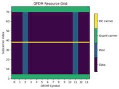
As can be seen in the figure above, the resource grid spans 76 subcarriers over 14 OFDM symbols. A DC guard carrier as well as some guard carriers to the left and right of the spectrum are nulled. The third and twelfth OFDM symbol are dedicated to pilot transmissions.
Let us now have a look at the pilot pattern used by the transmitter.
[5]:
rg.pilot_pattern.show();


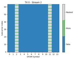

The pilot patterns are defined over the resource grid ofeffective subcarriers from which the nulled DC and guard carriers have been removed. This leaves us in our case with 76 - 1 (DC) - 5 (left guards) - 6 (right guards) = 64 effective subcarriers.
While the resource grid only knows which resource elements are reserved for pilots, it is the pilot pattern that defines what is actually transmitted on them. In our scenario, we have four transmit streams and configured theKroneckerPilotPattern. All streams use orthogonal pilot sequences, i.e., one pilot on every fourth subcarrier. You have full freedom to configure your ownPilotPattern.
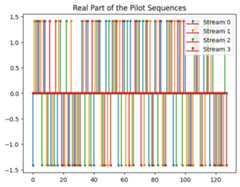
Let us now have a look at the actual pilot sequences for all streams which consists of random QPSK symbols. By default, the pilot sequences are normalized, such that the average power per pilot symbol is equal to one. As only every fourth pilot symbol in the sequence is used, their amplitude is scaled by a factor of two.
[6]:
plt.figure()plt.title("Real Part of the Pilot Sequences")foriinrange(num_streams_per_tx):plt.stem(np.real(rg.pilot_pattern.pilots[0,i]),markerfmt="C{}.".format(i),linefmt="C{}-".format(i),label="Stream{}".format(i))plt.legend()print("Average energy per pilot symbol:{:1.2f}".format(np.mean(np.abs(rg.pilot_pattern.pilots[0,0])**2)))
Average energy per pilot symbol: 1.00
Antenna Arrays
Next, we need to configure the antenna arrays used by the UT and BS. This can be ignored for simple channel models, such asAWGN,flat-fading,RayleighBlockFading, orTDL which do not account for antenna array geometries and antenna radiation patterns. However, other models, such asCDL,UMi,UMa, andRMa from the 3GPP 38.901 specification, require it.
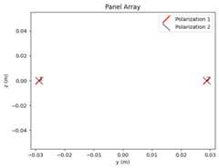
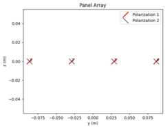
We will assume here that UT and BS antenna arrays are composed of dual cross-polarized antenna elements with an antenna pattern defined in the 3GPP 38.901 specification. By default, the antenna elements are spaced half of a wavelength apart in both vertical and horizontal directions. You can define your own antenna geometries an radiation patterns if needed.
AnAntennaArray is always defined in the y-z plane. It’s final orientation will be determined by the orientation of the UT or BS. This parameter can be configured in theChannelModel that we will create later.
[7]:
carrier_frequency=2.6e9# Carrier frequency in Hz.# This is needed here to define the antenna element spacing.ut_array=AntennaArray(num_rows=1,num_cols=int(num_ut_ant/2),polarization="dual",polarization_type="cross",antenna_pattern="38.901",carrier_frequency=carrier_frequency)ut_array.show()bs_array=AntennaArray(num_rows=1,num_cols=int(num_bs_ant/2),polarization="dual",polarization_type="cross",antenna_pattern="38.901",carrier_frequency=carrier_frequency)bs_array.show()
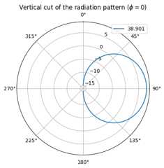
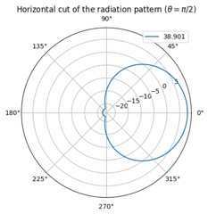
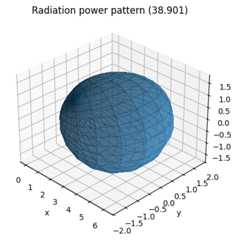
We can also visualize the radiation pattern of an individual antenna element:
[8]:
ut_array.show_element_radiation_pattern()
CDL Channel Model
Now, we will create an instance of the CDL channel model.
[9]:
delay_spread=300e-9# Nominal delay spread in [s]. Please see the CDL documentation# about how to choose this value.direction="uplink"# The `direction` determines if the UT or BS is transmitting.# In the `uplink`, the UT is transmitting.cdl_model="B"# Suitable values are ["A", "B", "C", "D", "E"]speed=10# UT speed [m/s]. BSs are always assumed to be fixed.# The direction of travel will chosen randomly within the x-y plane.# Configure a channel impulse reponse (CIR) generator for the CDL model.# cdl() will generate CIRs that can be converted to discrete time or discrete frequency.cdl=CDL(cdl_model,delay_spread,carrier_frequency,ut_array,bs_array,direction,min_speed=speed)
CIR Sampling Process
The instancecdl of theCDLChannelModel can be used to generate batches of random realizations of continuous-time channel impulse responses, consisting of complex gainsa and delaystau for each path. To account for time-varying channels, a channel impulse responses is sampled at thesampling_frequency fornum_time_samples samples. For more details on this, please have a look at theAPI documentation of the channel models.
In order to model the channel in the frequency domain, we neednum_ofdm_symbols samples that are taken once perofdm_symbol_duration, which corresponds to the length of an OFDM symbol plus the cyclic prefix.
[10]:
a,tau=cdl(batch_size=32,num_time_steps=rg.num_ofdm_symbols,sampling_frequency=1/rg.ofdm_symbol_duration)
a have shape[batchsize,num_rx,num_rx_ant,num_tx,num_tx_ant,num_paths,num_time_steps]tau have shape[batch_size,num_rx,num_tx,num_paths].[11]:
print("Shape of the path gains: ",a.shape)print("Shape of the delays:",tau.shape)
Shape of the path gains: (32, 1, 8, 1, 4, 23, 14)Shape of the delays: (32, 1, 1, 23)
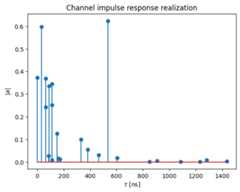
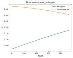
The delays are assumed to be static within the time-window of interest. Only the complex path gains change over time. The following two figures depict the channel impulse response at a particular time instant and the time-evolution of the gain of one path, respectively.
[12]:
plt.figure()plt.title("Channel impulse response realization")plt.stem(tau[0,0,0,:]/1e-9,np.abs(a)[0,0,0,0,0,:,0])plt.xlabel(r"$\tau$ [ns]")plt.ylabel(r"$|a|$")plt.figure()plt.title("Time evolution of path gain")plt.plot(np.arange(rg.num_ofdm_symbols)*rg.ofdm_symbol_duration/1e-6,np.real(a)[0,0,0,0,0,0,:])plt.plot(np.arange(rg.num_ofdm_symbols)*rg.ofdm_symbol_duration/1e-6,np.imag(a)[0,0,0,0,0,0,:])plt.legend(["Real part","Imaginary part"])plt.xlabel(r"$t$ [us]")plt.ylabel(r"$a$");
Generate the Channel Frequency Response
If we want to use the continuous-time channel impulse response to simulate OFDM transmissions under ideal conditions, i.e., no inter-symbol interference, inter-carrier interference, etc., we need to convert it to the frequency domain.
This can be done with the functioncir_to_ofdm_channel that computes the Fourier transform of the continuous-time channel impulse response at a set offrequencies, corresponding to the different subcarriers. The frequencies can be obtained with the help of the convenience functionsubcarrier_frequencies.
[13]:
frequencies=subcarrier_frequencies(rg.fft_size,rg.subcarrier_spacing)h_freq=cir_to_ofdm_channel(frequencies,a,tau,normalize=True)
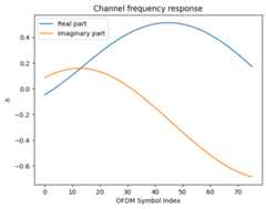
Let us have a look at the channel frequency response at a given time instant:
[14]:
plt.figure()plt.title("Channel frequency response")plt.plot(np.real(h_freq[0,0,0,0,0,0,:]))plt.plot(np.imag(h_freq[0,0,0,0,0,0,:]))plt.xlabel("OFDM Symbol Index")plt.ylabel(r"$h$")plt.legend(["Real part","Imaginary part"]);
We can apply the channel frequency response to a given input with theApplyOFDMChannel block. This block can also add additive white Gaussian noise (AWGN) to the channel output.
[15]:
# Function that will apply the channel frequency response to an input signalchannel_freq=ApplyOFDMChannel(add_awgn=True)
Generate the Discrete-Time Channel Impulse Response
In the same way as we have created the frequency channel impulse response from the continuous-time response, we can use the latter to compute a discrete-time impulse response. This can then be used to model the channel in the time-domain through discrete convolution with an input signal. Time-domain channel modeling is necessary whenever we want to deviate from the perfect OFDM scenario, e.g., OFDM without cyclic prefix, inter-subcarrier interference due to carrier-frequency offsets, phasenoise, or very high Doppler spread scenarios, as well as other single or multicarrier waveforms (OTFS, FBMC, UFMC, etc).
A discrete-time impulse response can be obtained with the help of the functioncir_to_time_channel that requires abandwidth parameter. This function first applies a perfect low-pass filter of the providedbandwith to the continuous-time channel impulse response and then samples the filtered response at the Nyquist rate. The resulting discrete-time impulse response is then truncated to finite length,depending on the delay spread.l_min andl_max denote truncation boundaries and the resulting channel hasl_tot=l_max-l_min+1 filter taps. A detailed mathematical description of this process is provided in the API documentation of the channel models. You can freely chose both parameters if you do not want to rely on the default values.
In order to model the channel in the domain, the continuous-time channel impulse response must be sampled at the Nyquist rate. We also need nownum_ofdm_symbolsx(fft_size+cyclic_prefix_length)+l_tot-1 samples in contrast tonum_ofdm_symbols samples for modeling in the frequency domain. This implies that the memory requirements of time-domain channel modeling is significantly higher. We therefore recommend to only use this feature if it is really necessary. Simulations with manytransmitters, receivers, and/or large antenna arrays become otherwise quickly prohibitively complex.
[16]:
# The following values for truncation are recommended.# Please feel free to tailor them to you needs.l_min,l_max=time_lag_discrete_time_channel(rg.bandwidth)l_tot=l_max-l_min+1a,tau=cdl(batch_size=2,num_time_steps=rg.num_time_samples+l_tot-1,sampling_frequency=rg.bandwidth)
[17]:
h_time=cir_to_time_channel(rg.bandwidth,a,tau,l_min=l_min,l_max=l_max,normalize=True)
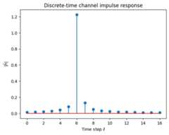
[18]:
plt.figure()plt.title("Discrete-time channel impulse response")plt.stem(np.abs(h_time[0,0,0,0,0,0]))plt.xlabel(r"Time step $\ell$")plt.ylabel(r"$|\bar{h}|$");
We can apply the discrete-time impulse response to a given input with theApplyTimeChannel block. This block can also add additive white Gaussian noise (AWGN) to the channel output.
[19]:
# Function that will apply the discrete-time channel impulse response to an input signalchannel_time=ApplyTimeChannel(rg.num_time_samples,l_tot=l_tot,add_awgn=True)
Other Physical Layer Components
Finally, we create instances of all other physical layer components we need. Most of these blocks are self-explanatory. For more information, please have a look at the API documentation.
[20]:
num_bits_per_symbol=2# QPSK modulationcoderate=0.5# Code raten=int(rg.num_data_symbols*num_bits_per_symbol)# Number of coded bitsk=int(n*coderate)# Number of information bits# The binary source will create batches of information bitsbinary_source=BinarySource()# The encoder maps information bits to coded bitsencoder=LDPC5GEncoder(k,n)# The mapper maps blocks of information bits to constellation symbolsmapper=Mapper("qam",num_bits_per_symbol)# The resource grid mapper maps symbols onto an OFDM resource gridrg_mapper=ResourceGridMapper(rg)# The zero forcing precoder precodes the transmit stream towards the intended antennaszf_precoder=RZFPrecoder(rg,sm,return_effective_channel=True)# OFDM modulator and demodulatormodulator=OFDMModulator(rg.cyclic_prefix_length)demodulator=OFDMDemodulator(rg.fft_size,l_min,rg.cyclic_prefix_length)# This function removes nulled subcarriers from any tensor having the shape of a resource gridremove_nulled_scs=RemoveNulledSubcarriers(rg)# The LS channel estimator will provide channel estimates and error variancesls_est=LSChannelEstimator(rg,interpolation_type="nn")# The LMMSE equalizer will provide soft symbols together with noise variance estimateslmmse_equ=LMMSEEqualizer(rg,sm)# The demapper produces LLR for all coded bitsdemapper=Demapper("app","qam",num_bits_per_symbol)# The decoder provides hard-decisions on the information bitsdecoder=LDPC5GDecoder(encoder,hard_out=True)
Simulations
Uplink Transmission in the Frequency Domain
Now, we will simulate our first uplink transmission! Inspect the code to understand how perfect CSI at the receiver can be simulated.
[21]:
batch_size=32# Depending on the memory of your GPU (or system when a CPU is used),# you can in(de)crease the batch size. The larger the batch size, the# more memory is required. However, simulations will also run much faster.ebno_db=40perfect_csi=False# Change to switch between perfect and imperfect CSI# Compute the noise power for a given Eb/No value.# This takes not only the coderate but also the overheads related pilot# transmissions and nulled carriersno=ebnodb2no(ebno_db,num_bits_per_symbol,coderate,rg)b=binary_source([batch_size,1,rg.num_streams_per_tx,encoder.k])c=encoder(b)x=mapper(c)x_rg=rg_mapper(x)# As explained above, we generate random batches of CIR, transform them# in the frequency domain and apply them to the resource grid in the# frequency domain.cir=cdl(batch_size,rg.num_ofdm_symbols,1/rg.ofdm_symbol_duration)h_freq=cir_to_ofdm_channel(frequencies,*cir,normalize=True)y=channel_freq(x_rg,h_freq,no)ifperfect_csi:# For perfect CSI, the receiver gets the channel frequency response as input# However, the channel estimator only computes estimates on the non-nulled# subcarriers. Therefore, we need to remove them here from `h_freq`.# This step can be skipped if no subcarriers are nulled.h_hat,err_var=remove_nulled_scs(h_freq),0.else:h_hat,err_var=ls_est(y,no)x_hat,no_eff=lmmse_equ(y,h_hat,err_var,no)llr=demapper(x_hat,no_eff)b_hat=decoder(llr)ber=compute_ber(b,b_hat)print("BER:{}".format(ber))
BER: 0.0
An alternative approach to simulations in the frequency domain is to use the convenience functionOFDMChannel that jointly generates and applies the channel frequency response. Using this function, we could have used the following code:
[22]:
ofdm_channel=OFDMChannel(cdl,rg,add_awgn=True,normalize_channel=True,return_channel=True)y,h_freq=ofdm_channel(x_rg,no)
Uplink Transmission in the Time Domain
In the previous example, OFDM modulation/demodulation were not needed as the entire system was simulated in the frequency domain. However, this modeling approach is not able to capture many realistic effects.
With the following modifications, the system can be modeled in the time domain.
Have a careful look at how perfect CSI of the channel frequency response is simulated here.
[23]:
batch_size=4# We pick a small batch_size as executing this code in Eager mode could consume a lot of memoryebno_db=30perfect_csi=Trueno=ebnodb2no(ebno_db,num_bits_per_symbol,coderate,rg)b=binary_source([batch_size,1,rg.num_streams_per_tx,encoder.k])c=encoder(b)x=mapper(c)x_rg=rg_mapper(x)# The CIR needs to be sampled every 1/bandwith [s].# In contrast to frequency-domain modeling, this implies# that the channel can change over the duration of a single# OFDM symbol. We now also need to simulate more# time steps.cir=cdl(batch_size,rg.num_time_samples+l_tot-1,rg.bandwidth)# OFDM modulation with cyclic prefix insertionx_time=modulator(x_rg)# Compute the discrete-time channel impulse reponseh_time=cir_to_time_channel(rg.bandwidth,*cir,l_min,l_max,normalize=True)# Compute the channel output# This computes the full convolution between the time-varying# discrete-time channel impulse reponse and the discrete-time# transmit signal. With this technique, the effects of an# insufficiently long cyclic prefix will become visible. This# is in contrast to frequency-domain modeling which imposes# no inter-symbol interfernce.y_time=channel_time(x_time,h_time,no)# OFDM demodulation and cyclic prefix removaly=demodulator(y_time)ifperfect_csi:a,tau=cir# We need to sub-sample the channel impulse reponse to compute perfect CSI# for the receiver as it only needs one channel realization per OFDM symbola_freq=a[...,rg.cyclic_prefix_length:-1:(rg.fft_size+rg.cyclic_prefix_length)]a_freq=a_freq[...,:rg.num_ofdm_symbols]# Compute the channel frequency responseh_freq=cir_to_ofdm_channel(frequencies,a_freq,tau,normalize=True)h_hat,err_var=remove_nulled_scs(h_freq),0.else:h_hat,err_var=ls_est(y,no)x_hat,no_eff=lmmse_equ(y,h_hat,err_var,no)llr=demapper(x_hat,no_eff)b_hat=decoder(llr)ber=compute_ber(b,b_hat)print("BER:{}".format(ber))
BER: 0.0
An alternative approach to simulations in the time domain is to use the convenience functionTimeChannel that jointly generates and applies the discrete-time channel impulse response. Using this function, we could have used the following code:
[24]:
time_channel=TimeChannel(cdl,rg.bandwidth,rg.num_time_samples,l_min=l_min,l_max=l_max,normalize_channel=True,add_awgn=True,return_channel=True)y_time,h_time=time_channel(x_time,no)
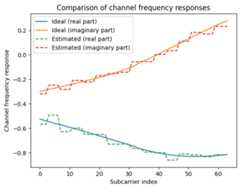
Next, we will compare the perfect CSI that we computed above using the ideal channel frequency response and the estimated channel response that we obtain from pilots with nearest-neighbor interpolation based on simulated transmissions in the time domain.
[25]:
# In the example above, we assumed perfect CSI, i.e.,# h_hat correpsond to the exact ideal channel frequency response.h_perf=h_hat[0,0,0,0,0,0]# We now compute the LS channel estimate from the pilots.h_est,_=ls_est(y,no)h_est=h_est[0,0,0,0,0,0]
[26]:
plt.figure()plt.plot(np.real(h_perf))plt.plot(np.imag(h_perf))plt.plot(np.real(h_est),"--")plt.plot(np.imag(h_est),"--")plt.xlabel("Subcarrier index")plt.ylabel("Channel frequency response")plt.legend(["Ideal (real part)","Ideal (imaginary part)","Estimated (real part)","Estimated (imaginary part)"]);plt.title("Comparison of channel frequency responses");
Downlink Transmission in the Frequency Domain
We will now simulate a simple downlink transmission in the frequency domain. In contrast to the uplink, the transmitter is now assumed to precode independent data streams to each antenna of the receiver based on perfect CSI.
The receiver can either estimate the channel or get access to the effective channel after precoding.
The first thing to do, is to change thedirection within the CDL model. This makes the BS the transmitter and the UT the receiver.
[27]:
direction="downlink"cdl=CDL(cdl_model,delay_spread,carrier_frequency,ut_array,bs_array,direction,min_speed=speed)
The following code shows the other necessary modifications:
[28]:
perfect_csi=True# Change to switch between perfect and imperfect CSIno=ebnodb2no(ebno_db,num_bits_per_symbol,coderate,rg)b=binary_source([batch_size,1,rg.num_streams_per_tx,encoder.k])c=encoder(b)x=mapper(c)x_rg=rg_mapper(x)cir=cdl(batch_size,rg.num_ofdm_symbols,1/rg.ofdm_symbol_duration)h_freq=cir_to_ofdm_channel(frequencies,*cir,normalize=True)# Precode the transmit signal in the frequency domain# It is here assumed that the transmitter has perfect knowledge of the channel# One could here reduce this to perfect knowledge of the channel for the first# OFDM symbol, or a noisy version of it to take outdated transmit CSI into account.# `g` is the post-beamforming or `effective channel` that can be# used to simulate perfect CSI at the receiver.x_rg,g=zf_precoder(x_rg,h_freq)y=channel_freq(x_rg,h_freq,no)ifperfect_csi:# The receiver gets here the effective channel after precoding as CSIh_hat,err_var=g,0.else:h_hat,err_var=ls_est(y,no)x_hat,no_eff=lmmse_equ(y,h_hat,err_var,no)llr=demapper(x_hat,no_eff)b_hat=decoder(llr)ber=compute_ber(b,b_hat)print("BER:{}".format(ber))
BER: 0.0
We do not explain here on purpose how to model the downlink transmission in the time domain as it is a good exercise for the reader to do it her/himself. The key steps are:
Sample the channel impulse response at the Nyquist rate.
Downsample it to the OFDM symbol (+ cyclic prefix) rate (look at the uplink example).
Convert the downsampled CIR to the frequency domain.
Give this CSI to the transmitter for precoding.
Convert the CIR to discrete-time to compute the channel output in the time domain.
Understand the Difference Between the CDL Models
Before we proceed with more advanced simulations, it is important to understand the differences between the different CDL models. The models “A”, “B”, and “C” are non-line-of-sight (NLOS) models, while “D” and “E” are LOS. In the following code snippet, we compute the empirical cummulative distribution function (CDF) of the condition number of the channel frequency response matrix between all receiver and transmit antennas.
[29]:
deffun(cdl_model):"""Generates a histogram of the channel condition numbers"""# Setup a CIR generatorcdl=CDL(cdl_model,delay_spread,carrier_frequency,ut_array,bs_array,"uplink",min_speed=0)# Generate random CIR realizations# As we nned only a single sample in time, the sampling_frequency# does not matter.cir=cdl(2000,1,1)# Compute the frequency responseh=cir_to_ofdm_channel(frequencies,*cir,normalize=True)# Reshape to [batch_size, fft_size, num_rx_ant, num_tx_ant]h=tf.squeeze(h)h=tf.transpose(h,[0,3,1,2])# Compute condition numberc=np.reshape(np.linalg.cond(h),[-1])# Compute normalized histogramhist,bins=np.histogram(c,150,(1,150))hist=hist/np.sum(hist)returnbins[:-1],histplt.figure()forcdl_modelin["A","B","C","D","E"]:bins,hist=fun(cdl_model)plt.plot(bins,np.cumsum(hist))plt.xlim([0,150])plt.legend(["CDL-A","CDL-B","CDL-C","CDL-D","CDL-E"]);plt.xlabel("Channel Condition Number")plt.ylabel("CDF")plt.title("CDF of the condition number of 8x4 MIMO channels");
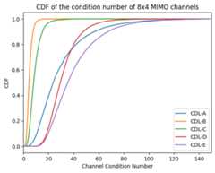
From the figure above, you can observe that the CDL-B and CDL-C models are substantially better conditioned than the other models. This makes them more suitable for MIMO transmissions as we will observe in the next section.
Create an End-to-End Model
For longer simulations, it is often convenient to pack all code into a single model that outputs batches of transmitted and received information bits at a given Eb/No point. The following code defines a very general model that can simulate uplink and downlink transmissions with time or frequency domain modeling over the different CDL models. It allows to configure perfect or imperfect CSI, UT speed, cyclic prefix length, and the number of OFDM symbols for pilot transmissions.
[30]:
classModel(Block):"""This block simulates OFDM MIMO transmissions over the CDL model. Simulates point-to-point transmissions between a UT and a BS. Uplink and downlink transmissions can be realized with either perfect CSI or channel estimation. ZF Precoding for downlink transmissions is assumed. The receiver (in both uplink and downlink) applies LS channel estimation and LMMSE MIMO equalization. A 5G LDPC code as well as QAM modulation are used. Parameters ---------- domain : One of ["time", "freq"], str Determines if the channel is modeled in the time or frequency domain. Time-domain simulations are generally slower and consume more memory. They allow modeling of inter-symbol interference and channel changes during the duration of an OFDM symbol. direction : One of ["uplink", "downlink"], str For "uplink", the UT transmits. For "downlink" the BS transmits. cdl_model : One of ["A", "B", "C", "D", "E"], str The CDL model to use. Note that "D" and "E" are LOS models that are not well suited for the transmissions of multiple streams. delay_spread : float The nominal delay spread [s]. perfect_csi : bool Indicates if perfect CSI at the receiver should be assumed. For downlink transmissions, the transmitter is always assumed to have perfect CSI. speed : float The UT speed [m/s]. cyclic_prefix_length : int The length of the cyclic prefix in number of samples. pilot_ofdm_symbol_indices : list, int List of integers defining the OFDM symbol indices that are reserved for pilots. subcarrier_spacing : float The subcarrier spacing [Hz]. Defaults to 15e3. Input ----- batch_size : int The batch size, i.e., the number of independent Mote Carlo simulations to be performed at once. The larger this number, the larger the memory requiremens. ebno_db : float The Eb/No [dB]. This value is converted to an equivalent noise power by taking the modulation order, coderate, pilot and OFDM-related overheads into account. Output ------ b : [batch_size, 1, num_streams, k], tf.float32 The tensor of transmitted information bits for each stream. b_hat : [batch_size, 1, num_streams, k], tf.float32 The tensor of received information bits for each stream. """def__init__(self,domain,direction,cdl_model,delay_spread,perfect_csi,speed,cyclic_prefix_length,pilot_ofdm_symbol_indices,subcarrier_spacing=15e3):super().__init__()# Provided parametersself._domain=domainself._direction=directionself._cdl_model=cdl_modelself._delay_spread=delay_spreadself._perfect_csi=perfect_csiself._speed=speedself._cyclic_prefix_length=cyclic_prefix_lengthself._pilot_ofdm_symbol_indices=pilot_ofdm_symbol_indices# System parametersself._carrier_frequency=2.6e9self._subcarrier_spacing=subcarrier_spacingself._fft_size=72self._num_ofdm_symbols=14self._num_ut_ant=4# Must be a multiple of two as dual-polarized antennas are usedself._num_bs_ant=8# Must be a multiple of two as dual-polarized antennas are usedself._num_streams_per_tx=self._num_ut_antself._dc_null=Trueself._num_guard_carriers=[5,6]self._pilot_pattern="kronecker"self._pilot_ofdm_symbol_indices=pilot_ofdm_symbol_indicesself._num_bits_per_symbol=2self._coderate=0.5# Required system componentsself._sm=StreamManagement(np.array([[1]]),self._num_streams_per_tx)self._rg=ResourceGrid(num_ofdm_symbols=self._num_ofdm_symbols,fft_size=self._fft_size,subcarrier_spacing=self._subcarrier_spacing,num_tx=1,num_streams_per_tx=self._num_streams_per_tx,cyclic_prefix_length=self._cyclic_prefix_length,num_guard_carriers=self._num_guard_carriers,dc_null=self._dc_null,pilot_pattern=self._pilot_pattern,pilot_ofdm_symbol_indices=self._pilot_ofdm_symbol_indices)self._n=int(self._rg.num_data_symbols*self._num_bits_per_symbol)self._k=int(self._n*self._coderate)self._ut_array=AntennaArray(num_rows=1,num_cols=int(self._num_ut_ant/2),polarization="dual",polarization_type="cross",antenna_pattern="38.901",carrier_frequency=self._carrier_frequency)self._bs_array=AntennaArray(num_rows=1,num_cols=int(self._num_bs_ant/2),polarization="dual",polarization_type="cross",antenna_pattern="38.901",carrier_frequency=self._carrier_frequency)self._cdl=CDL(model=self._cdl_model,delay_spread=self._delay_spread,carrier_frequency=self._carrier_frequency,ut_array=self._ut_array,bs_array=self._bs_array,direction=self._direction,min_speed=self._speed)self._frequencies=subcarrier_frequencies(self._rg.fft_size,self._rg.subcarrier_spacing)ifself._domain=="freq":self._channel_freq=ApplyOFDMChannel(add_awgn=True)elifself._domain=="time":self._l_min,self._l_max=time_lag_discrete_time_channel(self._rg.bandwidth)self._l_tot=self._l_max-self._l_min+1self._channel_time=ApplyTimeChannel(self._rg.num_time_samples,l_tot=self._l_tot,add_awgn=True)self._modulator=OFDMModulator(self._cyclic_prefix_length)self._demodulator=OFDMDemodulator(self._fft_size,self._l_min,self._cyclic_prefix_length)self._binary_source=BinarySource()self._encoder=LDPC5GEncoder(self._k,self._n)self._mapper=Mapper("qam",self._num_bits_per_symbol)self._rg_mapper=ResourceGridMapper(self._rg)ifself._direction=="downlink":self._zf_precoder=RZFPrecoder(self._rg,self._sm,return_effective_channel=True)self._ls_est=LSChannelEstimator(self._rg,interpolation_type="nn")self._lmmse_equ=LMMSEEqualizer(self._rg,self._sm)self._demapper=Demapper("app","qam",self._num_bits_per_symbol)self._decoder=LDPC5GDecoder(self._encoder,hard_out=True)self._remove_nulled_scs=RemoveNulledSubcarriers(self._rg)@tf.function# Run in graph mode. See the following guide: https://www.tensorflow.org/guide/functiondefcall(self,batch_size,ebno_db):no=ebnodb2no(ebno_db,self._num_bits_per_symbol,self._coderate,self._rg)b=self._binary_source([batch_size,1,self._num_streams_per_tx,self._k])c=self._encoder(b)x=self._mapper(c)x_rg=self._rg_mapper(x)ifself._domain=="time":# Time-domain simulationsa,tau=self._cdl(batch_size,self._rg.num_time_samples+self._l_tot-1,self._rg.bandwidth)h_time=cir_to_time_channel(self._rg.bandwidth,a,tau,l_min=self._l_min,l_max=self._l_max,normalize=True)# As precoding is done in the frequency domain, we need to downsample# the path gains `a` to the OFDM symbol rate prior to converting the CIR# to the channel frequency response.a_freq=a[...,self._rg.cyclic_prefix_length:-1:(self._rg.fft_size+self._rg.cyclic_prefix_length)]a_freq=a_freq[...,:self._rg.num_ofdm_symbols]h_freq=cir_to_ofdm_channel(self._frequencies,a_freq,tau,normalize=True)ifself._direction=="downlink":x_rg,g=self._zf_precoder(x_rg,h_freq)x_time=self._modulator(x_rg)y_time=self._channel_time(x_time,h_time,no)y=self._demodulator(y_time)elifself._domain=="freq":# Frequency-domain simulationscir=self._cdl(batch_size,self._rg.num_ofdm_symbols,1/self._rg.ofdm_symbol_duration)h_freq=cir_to_ofdm_channel(self._frequencies,*cir,normalize=True)ifself._direction=="downlink":x_rg,g=self._zf_precoder(x_rg,h_freq)y=self._channel_freq(x_rg,h_freq,no)ifself._perfect_csi:ifself._direction=="uplink":h_hat=self._remove_nulled_scs(h_freq)elifself._direction=="downlink":h_hat=gerr_var=0.0else:h_hat,err_var=self._ls_est(y,no)x_hat,no_eff=self._lmmse_equ(y,h_hat,err_var,no)llr=self._demapper(x_hat,no_eff)b_hat=self._decoder(llr)returnb,b_hat
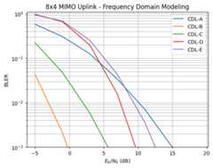
Compare Uplink Performance Over the Different CDL Models
We will now compare the uplink performance over the various CDL models assuming perfect CSI at the receiver. Note that these simulations might take some time depending or you available hardware. You can reduce thebatch_size if the model does not fit into the memory of your GPU. The code will also run on CPU if not GPU is available.
If you do not want to run the simulation your self, you skip the next cell and simply look at the result in the next cell.
[31]:
UL_SIMS={"ebno_db":list(np.arange(-5,20,4.0)),"cdl_model":["A","B","C","D","E"],"delay_spread":100e-9,"domain":"freq","direction":"uplink","perfect_csi":True,"speed":0.0,"cyclic_prefix_length":6,"pilot_ofdm_symbol_indices":[2,11],"ber":[],"bler":[],"duration":None}start=time.time()forcdl_modelinUL_SIMS["cdl_model"]:model=Model(domain=UL_SIMS["domain"],direction=UL_SIMS["direction"],cdl_model=cdl_model,delay_spread=UL_SIMS["delay_spread"],perfect_csi=UL_SIMS["perfect_csi"],speed=UL_SIMS["speed"],cyclic_prefix_length=UL_SIMS["cyclic_prefix_length"],pilot_ofdm_symbol_indices=UL_SIMS["pilot_ofdm_symbol_indices"])ber,bler=sim_ber(model,UL_SIMS["ebno_db"],batch_size=256,max_mc_iter=100,num_target_block_errors=1000,target_bler=1e-3)UL_SIMS["ber"].append(list(ber.numpy()))UL_SIMS["bler"].append(list(bler.numpy()))UL_SIMS["duration"]=time.time()-start
EbNo [dB] | BER | BLER | bit errors | num bits | block errors | num blocks | runtime [s] | status--------------------------------------------------------------------------------------------------------------------------------------- -5.0 | 1.1980e-01 | 5.7861e-01 | 176652 | 1474560 | 1185 | 2048 | 8.0 |reached target block errors -1.0 | 5.5480e-02 | 3.0542e-01 | 163616 | 2949120 | 1251 | 4096 | 0.6 |reached target block errors 3.0 | 1.9751e-02 | 1.2463e-01 | 116494 | 5898240 | 1021 | 8192 | 1.3 |reached target block errors 7.0 | 5.1353e-03 | 3.3708e-02 | 109798 | 21381120 | 1001 | 29696 | 4.6 |reached target block errors 11.0 | 9.5230e-04 | 7.0605e-03 | 70211 | 73728000 | 723 | 102400 | 15.9 |reached max iterations 15.0 | 1.1471e-04 | 9.9609e-04 | 8457 | 73728000 | 102 | 102400 | 15.8 |reached max iterationsSimulation stopped as target BLER is reached @ EbNo = 15.0 dB.EbNo [dB] | BER | BLER | bit errors | num bits | block errors | num blocks | runtime [s] | status--------------------------------------------------------------------------------------------------------------------------------------- -5.0 | 6.0769e-03 | 4.3648e-02 | 103049 | 16957440 | 1028 | 23552 | 6.4 |reached target block errors -1.0 | 2.4938e-04 | 2.0996e-03 | 18386 | 73728000 | 215 | 102400 | 15.9 |reached max iterations 3.0 | 2.5228e-06 | 3.9063e-05 | 186 | 73728000 | 4 | 102400 | 15.9 |reached max iterationsSimulation stopped as target BLER is reached @ EbNo = 3.0 dB.EbNo [dB] | BER | BLER | bit errors | num bits | block errors | num blocks | runtime [s] | status--------------------------------------------------------------------------------------------------------------------------------------- -5.0 | 3.8473e-02 | 2.2422e-01 | 141827 | 3686400 | 1148 | 5120 | 3.3 |reached target block errors -1.0 | 7.3453e-03 | 4.7852e-02 | 113727 | 15482880 | 1029 | 21504 | 3.4 |reached target block errors 3.0 | 7.9734e-04 | 5.7520e-03 | 58786 | 73728000 | 589 | 102400 | 16.3 |reached max iterations 7.0 | 4.9710e-05 | 4.0039e-04 | 3665 | 73728000 | 41 | 102400 | 16.5 |reached max iterationsSimulation stopped as target BLER is reached @ EbNo = 7.0 dB.EbNo [dB] | BER | BLER | bit errors | num bits | block errors | num blocks | runtime [s] | status--------------------------------------------------------------------------------------------------------------------------------------- -5.0 | 2.1653e-01 | 9.6631e-01 | 319293 | 1474560 | 1979 | 2048 | 2.9 |reached target block errors -1.0 | 1.1095e-01 | 6.6064e-01 | 163597 | 1474560 | 1353 | 2048 | 0.3 |reached target block errors 3.0 | 2.3985e-02 | 1.9570e-01 | 88420 | 3686400 | 1002 | 5120 | 0.7 |reached target block errors 7.0 | 1.5358e-03 | 1.5641e-02 | 71338 | 46448640 | 1009 | 64512 | 9.4 |reached target block errors 11.0 | 1.6995e-05 | 2.4414e-04 | 1253 | 73728000 | 25 | 102400 | 14.8 |reached max iterationsSimulation stopped as target BLER is reached @ EbNo = 11.0 dB.EbNo [dB] | BER | BLER | bit errors | num bits | block errors | num blocks | runtime [s] | status--------------------------------------------------------------------------------------------------------------------------------------- -5.0 | 2.1054e-01 | 9.3848e-01 | 310448 | 1474560 | 1922 | 2048 | 2.8 |reached target block errors -1.0 | 1.2151e-01 | 6.8311e-01 | 179170 | 1474560 | 1399 | 2048 | 0.3 |reached target block errors 3.0 | 3.4438e-02 | 2.5220e-01 | 101562 | 2949120 | 1033 | 4096 | 0.6 |reached target block errors 7.0 | 4.9951e-03 | 4.2926e-02 | 84704 | 16957440 | 1011 | 23552 | 3.5 |reached target block errors 11.0 | 3.4846e-04 | 3.5938e-03 | 25691 | 73728000 | 368 | 102400 | 15.0 |reached max iterations 15.0 | 1.1393e-05 | 1.2695e-04 | 840 | 73728000 | 13 | 102400 | 15.0 |reached max iterationsSimulation stopped as target BLER is reached @ EbNo = 15.0 dB.
[32]:
print("Simulation duration:{:1.2f} [h]".format(UL_SIMS["duration"]/3600))plt.figure()plt.xlabel(r"$E_b/N_0$ (dB)")plt.ylabel("BLER")plt.grid(which="both")plt.title("8x4 MIMO Uplink - Frequency Domain Modeling");plt.ylim([1e-3,1.1])legend=[]fori,blerinenumerate(UL_SIMS["bler"]):plt.semilogy(UL_SIMS["ebno_db"],bler)legend.append("CDL-{}".format(UL_SIMS["cdl_model"][i]))plt.legend(legend);
Simulation duration: 0.05 [h]
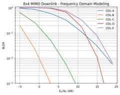
Compare Downlink Performance Over the Different CDL Models
We will now compare the downlink performance over the various CDL models assuming perfect CSI at the receiver.
If you do not want to run the simulation your self, you skip the next cell and simply look at the result in the next cell.
[33]:
DL_SIMS={"ebno_db":list(np.arange(-5,20,4.0)),"cdl_model":["A","B","C","D","E"],"delay_spread":100e-9,"domain":"freq","direction":"downlink","perfect_csi":True,"speed":0.0,"cyclic_prefix_length":6,"pilot_ofdm_symbol_indices":[2,11],"ber":[],"bler":[],"duration":None}start=time.time()forcdl_modelinDL_SIMS["cdl_model"]:model=Model(domain=DL_SIMS["domain"],direction=DL_SIMS["direction"],cdl_model=cdl_model,delay_spread=DL_SIMS["delay_spread"],perfect_csi=DL_SIMS["perfect_csi"],speed=DL_SIMS["speed"],cyclic_prefix_length=DL_SIMS["cyclic_prefix_length"],pilot_ofdm_symbol_indices=DL_SIMS["pilot_ofdm_symbol_indices"])ber,bler=sim_ber(model,DL_SIMS["ebno_db"],batch_size=256,max_mc_iter=100,num_target_block_errors=1000,target_bler=1e-3)DL_SIMS["ber"].append(list(ber.numpy()))DL_SIMS["bler"].append(list(bler.numpy()))DL_SIMS["duration"]=time.time()-start
EbNo [dB] | BER | BLER | bit errors | num bits | block errors | num blocks | runtime [s] | status--------------------------------------------------------------------------------------------------------------------------------------- -5.0 | 3.5490e-01 | 9.7217e-01 | 523322 | 1474560 | 1991 | 2048 | 3.3 |reached target block errors -1.0 | 2.7378e-01 | 8.5059e-01 | 403709 | 1474560 | 1742 | 2048 | 0.4 |reached target block errors 3.0 | 1.6477e-01 | 5.9473e-01 | 242964 | 1474560 | 1218 | 2048 | 0.3 |reached target block errors 7.0 | 8.0808e-02 | 3.2373e-01 | 238313 | 2949120 | 1326 | 4096 | 0.7 |reached target block errors 11.0 | 2.4723e-02 | 1.0959e-01 | 164051 | 6635520 | 1010 | 9216 | 1.6 |reached target block errors 15.0 | 6.0848e-03 | 3.0244e-02 | 148044 | 24330240 | 1022 | 33792 | 5.8 |reached target block errors 19.0 | 1.0187e-03 | 5.6055e-03 | 75109 | 73728000 | 574 | 102400 | 17.6 |reached max iterationsEbNo [dB] | BER | BLER | bit errors | num bits | block errors | num blocks | runtime [s] | status--------------------------------------------------------------------------------------------------------------------------------------- -5.0 | 3.5875e-02 | 2.0000e-01 | 132249 | 3686400 | 1024 | 5120 | 3.6 |reached target block errors -1.0 | 3.4401e-03 | 2.1527e-02 | 116672 | 33914880 | 1014 | 47104 | 8.3 |reached target block errors 3.0 | 1.2263e-04 | 9.5703e-04 | 9041 | 73728000 | 98 | 102400 | 17.9 |reached max iterationsSimulation stopped as target BLER is reached @ EbNo = 3.0 dB.EbNo [dB] | BER | BLER | bit errors | num bits | block errors | num blocks | runtime [s] | status--------------------------------------------------------------------------------------------------------------------------------------- -5.0 | 1.6116e-01 | 6.5039e-01 | 237638 | 1474560 | 1332 | 2048 | 3.1 |reached target block errors -1.0 | 5.1945e-02 | 2.4829e-01 | 153192 | 2949120 | 1017 | 4096 | 0.7 |reached target block errors 3.0 | 9.2209e-03 | 5.0293e-02 | 135968 | 14745600 | 1030 | 20480 | 3.5 |reached target block errors 7.0 | 9.2379e-04 | 5.5469e-03 | 68109 | 73728000 | 568 | 102400 | 17.7 |reached max iterations 11.0 | 5.1731e-05 | 3.1250e-04 | 3814 | 73728000 | 32 | 102400 | 17.7 |reached max iterationsSimulation stopped as target BLER is reached @ EbNo = 11.0 dB.EbNo [dB] | BER | BLER | bit errors | num bits | block errors | num blocks | runtime [s] | status--------------------------------------------------------------------------------------------------------------------------------------- -5.0 | 4.1748e-01 | 1.0000e+00 | 307799 | 737280 | 1024 | 1024 | 3.2 |reached target block errors -1.0 | 3.6759e-01 | 9.9902e-01 | 271019 | 737280 | 1023 | 1024 | 0.2 |reached target block errors 3.0 | 2.8536e-01 | 9.5508e-01 | 420775 | 1474560 | 1956 | 2048 | 0.3 |reached target block errors 7.0 | 1.4852e-01 | 6.6943e-01 | 219003 | 1474560 | 1371 | 2048 | 0.3 |reached target block errors 11.0 | 3.0269e-02 | 1.7285e-01 | 133899 | 4423680 | 1062 | 6144 | 1.0 |reached target block errors 15.0 | 1.5454e-03 | 1.0927e-02 | 102543 | 66355200 | 1007 | 92160 | 14.8 |reached target block errors 19.0 | 3.8113e-06 | 4.8828e-05 | 281 | 73728000 | 5 | 102400 | 16.5 |reached max iterationsSimulation stopped as target BLER is reached @ EbNo = 19.0 dB.EbNo [dB] | BER | BLER | bit errors | num bits | block errors | num blocks | runtime [s] | status--------------------------------------------------------------------------------------------------------------------------------------- -5.0 | 4.2295e-01 | 1.0000e+00 | 311833 | 737280 | 1024 | 1024 | 2.9 |reached target block errors -1.0 | 3.8416e-01 | 9.9902e-01 | 283236 | 737280 | 1023 | 1024 | 0.2 |reached target block errors 3.0 | 3.1512e-01 | 9.7510e-01 | 464664 | 1474560 | 1997 | 2048 | 0.3 |reached target block errors 7.0 | 1.9181e-01 | 7.3730e-01 | 282832 | 1474560 | 1510 | 2048 | 0.3 |reached target block errors 11.0 | 7.0916e-02 | 3.2780e-01 | 156855 | 2211840 | 1007 | 3072 | 0.5 |reached target block errors 15.0 | 1.3874e-02 | 7.6730e-02 | 143210 | 10321920 | 1100 | 14336 | 2.3 |reached target block errors 19.0 | 9.7325e-04 | 6.3281e-03 | 71756 | 73728000 | 648 | 102400 | 16.6 |reached max iterations
[34]:
print("Simulation duration:{:1.2f} [h]".format(DL_SIMS["duration"]/3600))plt.figure()plt.xlabel(r"$E_b/N_0$ (dB)")plt.ylabel("BLER")plt.grid(which="both")plt.title("8x4 MIMO Downlink - Frequency Domain Modeling");plt.ylim([1e-3,1.1])legend=[]fori,blerinenumerate(DL_SIMS["bler"]):plt.semilogy(DL_SIMS["ebno_db"],bler)legend.append("CDL-{}".format(DL_SIMS["cdl_model"][i]))plt.legend(legend);
Simulation duration: 0.05 [h]
Evaluate the Impact of Mobility
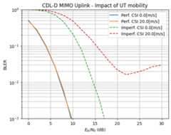
Let us now have a look at the impact of the UT speed on the uplink performance. We compare the scenarios of perfect and imperfect CSI and 0 m/s and 20 m/s speed. To amplify the detrimental effects of high mobility, we only configure a single OFDM symbol for pilot transmissions at the beginning of the resource grid. With perfect CSI, mobility plays hardly any role. However, once channel estimation is taken into acount, the BLER saturates.
If you do not want to run the simulation your self, you skip the next cell and simply look at the result in the next cell.
[35]:
MOBILITY_SIMS={"ebno_db":list(np.arange(0,32,2.0)),"cdl_model":"D","delay_spread":100e-9,"domain":"freq","direction":"uplink","perfect_csi":[True,False],"speed":[0.0,20.0],"cyclic_prefix_length":6,"pilot_ofdm_symbol_indices":[0],"ber":[],"bler":[],"duration":None}start=time.time()forperfect_csiinMOBILITY_SIMS["perfect_csi"]:forspeedinMOBILITY_SIMS["speed"]:model=Model(domain=MOBILITY_SIMS["domain"],direction=MOBILITY_SIMS["direction"],cdl_model=MOBILITY_SIMS["cdl_model"],delay_spread=MOBILITY_SIMS["delay_spread"],perfect_csi=perfect_csi,speed=speed,cyclic_prefix_length=MOBILITY_SIMS["cyclic_prefix_length"],pilot_ofdm_symbol_indices=MOBILITY_SIMS["pilot_ofdm_symbol_indices"])ber,bler=sim_ber(model,MOBILITY_SIMS["ebno_db"],batch_size=256,max_mc_iter=100,num_target_block_errors=1000,target_bler=1e-3)MOBILITY_SIMS["ber"].append(list(ber.numpy()))MOBILITY_SIMS["bler"].append(list(bler.numpy()))MOBILITY_SIMS["duration"]=time.time()-start
EbNo [dB] | BER | BLER | bit errors | num bits | block errors | num blocks | runtime [s] | status--------------------------------------------------------------------------------------------------------------------------------------- 0.0 | 7.2939e-02 | 5.0879e-01 | 116516 | 1597440 | 1042 | 2048 | 3.1 |reached target block errors 2.0 | 3.1453e-02 | 2.5513e-01 | 100488 | 3194880 | 1045 | 4096 | 0.6 |reached target block errors 4.0 | 1.0154e-02 | 9.5259e-02 | 89208 | 8785920 | 1073 | 11264 | 1.7 |reached target block errors 6.0 | 2.5844e-03 | 2.6895e-02 | 76377 | 29552640 | 1019 | 37888 | 5.7 |reached target block errors 8.0 | 4.3483e-04 | 4.8633e-03 | 34731 | 79872000 | 498 | 102400 | 15.4 |reached max iterations 10.0 | 6.2500e-05 | 8.0078e-04 | 4992 | 79872000 | 82 | 102400 | 15.4 |reached max iterationsSimulation stopped as target BLER is reached @ EbNo = 10.0 dB.EbNo [dB] | BER | BLER | bit errors | num bits | block errors | num blocks | runtime [s] | status--------------------------------------------------------------------------------------------------------------------------------------- 0.0 | 7.1526e-02 | 4.8828e-01 | 114259 | 1597440 | 1000 | 2048 | 2.8 |reached target block errors 2.0 | 3.3917e-02 | 2.6831e-01 | 108361 | 3194880 | 1099 | 4096 | 0.6 |reached target block errors 4.0 | 1.1291e-02 | 9.9707e-02 | 90180 | 7987200 | 1021 | 10240 | 1.5 |reached target block errors 6.0 | 2.7696e-03 | 2.7479e-02 | 79637 | 28753920 | 1013 | 36864 | 5.5 |reached target block errors 8.0 | 4.7180e-04 | 5.5371e-03 | 37684 | 79872000 | 567 | 102400 | 15.3 |reached max iterations 10.0 | 4.2393e-05 | 6.2500e-04 | 3386 | 79872000 | 64 | 102400 | 15.4 |reached max iterationsSimulation stopped as target BLER is reached @ EbNo = 10.0 dB.EbNo [dB] | BER | BLER | bit errors | num bits | block errors | num blocks | runtime [s] | status--------------------------------------------------------------------------------------------------------------------------------------- 0.0 | 2.6249e-01 | 9.9316e-01 | 209659 | 798720 | 1017 | 1024 | 3.0 |reached target block errors 2.0 | 2.4350e-01 | 9.7021e-01 | 388974 | 1597440 | 1987 | 2048 | 0.3 |reached target block errors 4.0 | 2.0585e-01 | 8.9404e-01 | 328834 | 1597440 | 1831 | 2048 | 0.3 |reached target block errors 6.0 | 1.4909e-01 | 7.1387e-01 | 238158 | 1597440 | 1462 | 2048 | 0.3 |reached target block errors 8.0 | 8.4108e-02 | 4.5312e-01 | 201537 | 2396160 | 1392 | 3072 | 0.5 |reached target block errors 10.0 | 3.6978e-02 | 2.1289e-01 | 147675 | 3993600 | 1090 | 5120 | 0.8 |reached target block errors 12.0 | 1.2211e-02 | 7.5684e-02 | 136542 | 11182080 | 1085 | 14336 | 2.2 |reached target block errors 14.0 | 2.3035e-03 | 1.5861e-02 | 114070 | 49520640 | 1007 | 63488 | 9.6 |reached target block errors 16.0 | 4.4387e-04 | 3.2031e-03 | 35453 | 79872000 | 328 | 102400 | 15.4 |reached max iterations 18.0 | 4.5936e-05 | 3.7109e-04 | 3669 | 79872000 | 38 | 102400 | 15.4 |reached max iterationsSimulation stopped as target BLER is reached @ EbNo = 18.0 dB.EbNo [dB] | BER | BLER | bit errors | num bits | block errors | num blocks | runtime [s] | status--------------------------------------------------------------------------------------------------------------------------------------- 0.0 | 2.7444e-01 | 9.9902e-01 | 219198 | 798720 | 1023 | 1024 | 2.9 |reached target block errors 2.0 | 2.5494e-01 | 9.8730e-01 | 203622 | 798720 | 1011 | 1024 | 0.2 |reached target block errors 4.0 | 2.3164e-01 | 9.5215e-01 | 370027 | 1597440 | 1950 | 2048 | 0.3 |reached target block errors 6.0 | 1.8992e-01 | 8.4521e-01 | 303379 | 1597440 | 1731 | 2048 | 0.3 |reached target block errors 8.0 | 1.4158e-01 | 6.8750e-01 | 226160 | 1597440 | 1408 | 2048 | 0.3 |reached target block errors 10.0 | 9.3948e-02 | 4.8926e-01 | 150076 | 1597440 | 1002 | 2048 | 0.3 |reached target block errors 12.0 | 4.8350e-02 | 2.7563e-01 | 154472 | 3194880 | 1129 | 4096 | 0.7 |reached target block errors 14.0 | 2.5454e-02 | 1.5737e-01 | 142312 | 5591040 | 1128 | 7168 | 1.1 |reached target block errors 16.0 | 1.1697e-02 | 7.9477e-02 | 121451 | 10383360 | 1058 | 13312 | 2.1 |reached target block errors 18.0 | 4.9192e-03 | 3.9688e-02 | 98226 | 19968000 | 1016 | 25600 | 4.0 |reached target block errors 20.0 | 2.0987e-03 | 2.1888e-02 | 77107 | 36741120 | 1031 | 47104 | 7.3 |reached target block errors 22.0 | 9.8481e-04 | 1.6281e-02 | 47982 | 48721920 | 1017 | 62464 | 9.7 |reached target block errors 24.0 | 9.6179e-04 | 1.8338e-02 | 41483 | 43130880 | 1014 | 55296 | 8.5 |reached target block errors 26.0 | 1.4267e-03 | 2.1484e-02 | 52417 | 36741120 | 1012 | 47104 | 7.2 |reached target block errors 28.0 | 2.0896e-03 | 2.7027e-02 | 61752 | 29552640 | 1024 | 37888 | 5.7 |reached target block errors 30.0 | 2.6936e-03 | 2.9800e-02 | 70996 | 26357760 | 1007 | 33792 | 5.1 |reached target block errors
[36]:
print("Simulation duration:{:1.2f} [h]".format(MOBILITY_SIMS["duration"]/3600))plt.figure()plt.xlabel(r"$E_b/N_0$ (dB)")plt.ylabel("BLER")plt.grid(which="both")plt.title("CDL-D MIMO Uplink - Impact of UT mobility")i=0forperfect_csiinMOBILITY_SIMS["perfect_csi"]:forspeedinMOBILITY_SIMS["speed"]:style="{}".format("-"ifperfect_csielse"--")s="{} CSI{}[m/s]".format("Perf."ifperfect_csielse"Imperf.",speed)plt.semilogy(MOBILITY_SIMS["ebno_db"],MOBILITY_SIMS["bler"][i],style,label=s,)i+=1plt.legend();plt.ylim([1e-3,1]);
Simulation duration: 0.05 [h]
Evaluate the Impact of Insufficient Cyclic Prefix Length
As a final example, let us have a look at how to simulate OFDM with an insufficiently long cyclic prefix.
It is important to notice, that ISI cannot be simulated in the frequency domain as theOFDMChannel implicitly assumes perfectly synchronized and ISI-free transmissions. Having no cyclic prefix translates simply into an improved Eb/No as no energy for its transmission is used.
Simulating a channel in the time domain requires significantly more memory and compute which might limit the scenarios for which it can be used.
If you do not want to run the simulation your self, you skip the next cell and simply look at the result in the next cell.If you do not want to run the simulation your self, you skip the next cell and visualize the result in the next cell.
[37]:
CP_SIMS={"ebno_db":list(np.arange(0,17,2.0)),"cdl_model":"C","delay_spread":100e-9,"subcarrier_spacing":15e3,"domain":["freq","time"],"direction":"uplink","perfect_csi":False,"speed":3.0,"cyclic_prefix_length":[20,2],"pilot_ofdm_symbol_indices":[2,11],"ber":[],"bler":[],"duration":None}start=time.time()forcyclic_prefix_lengthinCP_SIMS["cyclic_prefix_length"]:fordomaininCP_SIMS["domain"]:model=Model(domain=domain,direction=CP_SIMS["direction"],cdl_model=CP_SIMS["cdl_model"],delay_spread=CP_SIMS["delay_spread"],perfect_csi=CP_SIMS["perfect_csi"],speed=CP_SIMS["speed"],cyclic_prefix_length=cyclic_prefix_length,pilot_ofdm_symbol_indices=CP_SIMS["pilot_ofdm_symbol_indices"],subcarrier_spacing=CP_SIMS["subcarrier_spacing"])ber,bler=sim_ber(model,CP_SIMS["ebno_db"],batch_size=64,max_mc_iter=1000,num_target_block_errors=1000,target_bler=1e-3)CP_SIMS["ber"].append(list(ber.numpy()))CP_SIMS["bler"].append(list(bler.numpy()))CP_SIMS["duration"]=time.time()-start
EbNo [dB] | BER | BLER | bit errors | num bits | block errors | num blocks | runtime [s] | status--------------------------------------------------------------------------------------------------------------------------------------- 0.0 | 5.8877e-02 | 2.8683e-01 | 151931 | 2580480 | 1028 | 3584 | 3.6 |reached target block errors 2.0 | 3.2954e-02 | 1.6504e-01 | 145776 | 4423680 | 1014 | 6144 | 1.6 |reached target block errors 4.0 | 1.4063e-02 | 7.3568e-02 | 139973 | 9953280 | 1017 | 13824 | 3.7 |reached target block errors 6.0 | 5.5723e-03 | 3.0228e-02 | 133521 | 23961600 | 1006 | 33280 | 8.9 |reached target block errors 8.0 | 2.1439e-03 | 1.2143e-02 | 127243 | 59351040 | 1001 | 82432 | 21.9 |reached target block errors 10.0 | 5.9717e-04 | 3.4492e-03 | 110070 | 184320000 | 883 | 256000 | 67.9 |reached max iterations 12.0 | 1.8627e-04 | 1.1055e-03 | 34334 | 184320000 | 283 | 256000 | 67.8 |reached max iterations 14.0 | 4.0679e-05 | 2.5000e-04 | 7498 | 184320000 | 64 | 256000 | 67.7 |reached max iterationsSimulation stopped as target BLER is reached @ EbNo = 14.0 dB.EbNo [dB] | BER | BLER | bit errors | num bits | block errors | num blocks | runtime [s] | status--------------------------------------------------------------------------------------------------------------------------------------- 0.0 | 6.7696e-02 | 3.1160e-01 | 162210 | 2396160 | 1037 | 3328 | 6.5 |reached target block errors 2.0 | 3.0083e-02 | 1.5595e-01 | 144168 | 4792320 | 1038 | 6656 | 4.7 |reached target block errors 4.0 | 1.4150e-02 | 7.5120e-02 | 135621 | 9584640 | 1000 | 13312 | 9.4 |reached target block errors 6.0 | 5.3648e-03 | 2.9998e-02 | 129539 | 24145920 | 1006 | 33536 | 23.8 |reached target block errors 8.0 | 1.9081e-03 | 1.0842e-02 | 126961 | 66539520 | 1002 | 92416 | 65.9 |reached target block errors 10.0 | 6.1646e-04 | 3.5859e-03 | 113625 | 184320000 | 918 | 256000 | 182.5 |reached max iterations 12.0 | 1.9007e-04 | 1.0781e-03 | 35034 | 184320000 | 276 | 256000 | 182.6 |reached max iterations 14.0 | 4.1130e-05 | 2.6563e-04 | 7581 | 184320000 | 68 | 256000 | 182.6 |reached max iterationsSimulation stopped as target BLER is reached @ EbNo = 14.0 dB.EbNo [dB] | BER | BLER | bit errors | num bits | block errors | num blocks | runtime [s] | status--------------------------------------------------------------------------------------------------------------------------------------- 0.0 | 4.5926e-02 | 2.2830e-01 | 152370 | 3317760 | 1052 | 4608 | 3.8 |reached target block errors 2.0 | 2.2464e-02 | 1.1500e-01 | 140780 | 6266880 | 1001 | 8704 | 2.3 |reached target block errors 4.0 | 9.6553e-03 | 5.0531e-02 | 138814 | 14376960 | 1009 | 19968 | 5.2 |reached target block errors 6.0 | 3.4924e-03 | 1.9415e-02 | 130033 | 37232640 | 1004 | 51712 | 13.4 |reached target block errors 8.0 | 1.1323e-03 | 6.4566e-03 | 126272 | 111513600 | 1000 | 154880 | 40.3 |reached target block errors 10.0 | 3.4135e-04 | 2.0000e-03 | 62917 | 184320000 | 512 | 256000 | 66.6 |reached max iterations 12.0 | 7.9986e-05 | 4.6875e-04 | 14743 | 184320000 | 120 | 256000 | 66.7 |reached max iterationsSimulation stopped as target BLER is reached @ EbNo = 12.0 dB.EbNo [dB] | BER | BLER | bit errors | num bits | block errors | num blocks | runtime [s] | status--------------------------------------------------------------------------------------------------------------------------------------- 0.0 | 1.1951e-01 | 5.3809e-01 | 176225 | 1474560 | 1102 | 2048 | 4.1 |reached target block errors 2.0 | 8.0203e-02 | 3.7678e-01 | 162614 | 2027520 | 1061 | 2816 | 1.8 |reached target block errors 4.0 | 4.8896e-02 | 2.4035e-01 | 153212 | 3133440 | 1046 | 4352 | 2.7 |reached target block errors 6.0 | 2.6285e-02 | 1.3385e-01 | 145343 | 5529600 | 1028 | 7680 | 4.8 |reached target block errors 8.0 | 1.1158e-02 | 5.9718e-02 | 135737 | 12165120 | 1009 | 16896 | 10.6 |reached target block errors 10.0 | 5.0670e-03 | 2.8448e-02 | 128886 | 25436160 | 1005 | 35328 | 22.2 |reached target block errors 12.0 | 1.9637e-03 | 1.2724e-02 | 111121 | 56586240 | 1000 | 78592 | 49.4 |reached target block errors 14.0 | 7.0154e-04 | 6.8189e-03 | 74223 | 105799680 | 1002 | 146944 | 92.6 |reached target block errors 16.0 | 1.9807e-04 | 5.8829e-03 | 24242 | 122388480 | 1000 | 169984 | 106.9 |reached target block errors
[38]:
print("Simulation duration:{:1.2f} [h]".format(CP_SIMS["duration"]/3600))plt.figure()plt.xlabel(r"$E_b/N_0$ (dB)")plt.ylabel("BLER")plt.grid(which="both")plt.title("CDL-B MIMO Uplink - Impact of Cyclic Prefix Length")i=0forcyclic_prefix_lengthinCP_SIMS["cyclic_prefix_length"]:fordomaininCP_SIMS["domain"]:s="{} Domain, CP length:{}".format("Freq"ifdomain=="freq"else"Time",cyclic_prefix_length)plt.semilogy(CP_SIMS["ebno_db"],CP_SIMS["bler"][i],label=s)i+=1plt.legend();plt.ylim([1e-3,1]);
Simulation duration: 0.39 [h]
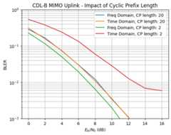
One can make a few important observations from the figure above:
The length of the cyclic prefix has no impact on the performance if the system is simulated in the frequency domain.The reason why the two curves for both frequency-domain simulations do not overlap is that the cyclic prefix length affects the way the Eb/No is computed.
With a sufficiently large cyclic prefix (in our case
cyclic_prefix_length=20>=l_tot=17), the performance of time and frequency-domain simulations are identical.With a too small cyclic prefix length, the performance degrades. At high SNR, inter-symbol interference (from multiple streams) becomes the dominating source of interference.