Power Control
This tutorial demonstrates how to allocate transmission power on a per-user basis in a 3GPP-compliant multicell scenario in the uplink and downlink direction.
Uplink: Implemented by theopen_loop_uplink_power_control function.This follows the open-loop power allocation procedure in 3GPP TS 38.213[1], where the transmit power partially compensate for the pathloss by a factor\(\alpha\in[0;1]\) while targeting a received power of\(P_0\) [dBm];
Downlink: Handled by thedownlink_fair_power_control function. This function maximizes a fairness function of the attainable throughput across the users on a per-sector basis.
Imports
We start by importing Sionna and the relevant external libraries:
[1]:
importosos.environ['TF_CPP_MIN_LOG_LEVEL']='3'ifos.getenv("CUDA_VISIBLE_DEVICES")isNone:gpu_num=0# Use "" to use the CPUifgpu_num!="":print(f'\nUsing GPU{gpu_num}\n')else:print('\nUsing CPU\n')os.environ["CUDA_VISIBLE_DEVICES"]=f"{gpu_num}"# Import Sionnatry:importsionna.sysexceptImportErrorase:importsysif'google.colab'insys.modules:# Install Sionna in Google Colabprint("Installing Sionna and restarting the runtime. Please run the cell again.")os.system("pip install sionna")os.kill(os.getpid(),5)else:raisee# Configure the notebook to use only a single GPU and allocate only as much memory as needed# For more details, see https://www.tensorflow.org/guide/gpuimporttensorflowastftf.get_logger().setLevel('ERROR')gpus=tf.config.list_physical_devices('GPU')ifgpus:try:tf.config.experimental.set_memory_growth(gpus[0],True)exceptRuntimeErrorase:print(e)
[2]:
# Additional external librariesimportmatplotlib.pyplotaspltimportnumpyasnp# Sionna componentsfromsionna.phy.utilsimportlog2,dbm_to_watt,watt_to_dbmfromsionna.phy.constantsimportBOLTZMANN_CONSTANTfromsionna.phy.channelimportGenerateOFDMChannelfromsionna.phy.ofdmimportResourceGrid,RZFPrecodedChannel, \EyePrecodedChannel,LMMSEPostEqualizationSINRfromsionna.phy.channel.tr38901importUMi,PanelArrayfromsionna.phy.mimoimportStreamManagementfromsionna.sysimportgen_hexgrid_topology, \downlink_fair_power_control,open_loop_uplink_power_controlfromsionna.sys.utilsimportspread_across_subcarriers,get_pathloss# Internal computational precisionsionna.phy.config.precision='single'# 'single' or 'double'# Set random seed for reproducibilitysionna.phy.config.seed=45
Multicell scenario
We first create a multicell 3GPP-compliant scenario on which power control will be performed in both the uplink and downlink directions.
Simulation Parameters
We define the main simulation parameters, including the topology settings, OFDM resource grid, and transmission power for the base stations and user terminal.
[3]:
# Number of independent scenariosbatch_size=1# Number of rings of the spiral hexagonal gridnum_rings=1# Number of co-scheduled users per sectornum_ut_per_sector=5# OFDM resource gridnum_ofdm_sym=10num_subcarriers=32subcarrier_spacing=15e3# [Hz]carrier_frequency=3.5e9# [Hz]# Base station and user terminal transmit powerbs_max_power_dbm=46# [dBm]ut_max_power_dbm=26# [dBm]# Convert power to Wattsut_max_power=dbm_to_watt(ut_max_power_dbm)# [W]bs_max_power=dbm_to_watt(bs_max_power_dbm)# [W]# Environment temperaturetemperature=294# [K]# Noise power per subcarrierno=BOLTZMANN_CONSTANT*temperature*subcarrier_spacing# Max distance between user terminal and serving base stationmax_bs_ut_dist=80# [m]
Antenna patterns
We create the antenna patterns for base stations and user terminals.
[4]:
# Create antenna arraysbs_array=PanelArray(num_rows_per_panel=3,num_cols_per_panel=2,polarization='dual',polarization_type='VH',antenna_pattern='38.901',carrier_frequency=carrier_frequency)ut_array=PanelArray(num_rows_per_panel=1,num_cols_per_panel=1,polarization='single',polarization_type='V',antenna_pattern='omni',carrier_frequency=carrier_frequency)num_ut_ant=ut_array.num_antnum_bs_ant=bs_array.num_ant
Topology
Next, we position base stations on a hexagonal grid according to a 3GPP-compliant scenario and randomly distribute users uniformly in each sector.
For more details on the generation of the topology, see theHexagonal Grid Topology notebook.
[5]:
# Generate the spiral hexagonal grid topologytopology=gen_hexgrid_topology(batch_size=batch_size,num_rings=num_rings,num_ut_per_sector=num_ut_per_sector,max_bs_ut_dist=max_bs_ut_dist,scenario='umi')ut_loc,bs_loc,*_=topology# N. users and base stationsnum_bs=bs_loc.shape[1]num_ut=ut_loc.shape[1]# In the uplink, the user is the transmitter and the base station is the receivernum_rx,num_tx=num_bs,num_ut
We set and compute the number of streams per user and base station, respectively.
[6]:
# Set number of streams per usernum_streams_per_ut=num_ut_ant# Number of streams per base stationnum_streams_per_bs=num_streams_per_ut*num_ut_per_sectorassertnum_streams_per_ut<=num_ut_ant, \"The # of streams per user must not exceed the # of its antennas"
Each receiver is associated with its serving base station.
[7]:
# For simplicity, each user is associated with its nearest base station# Uplink# RX-TX association matrixrx_tx_association_ul=np.zeros([num_rx,num_tx])idx_fair=np.array([[i1,i2]fori1inrange(num_rx)fori2innp.arange(i1*num_ut_per_sector,(i1+1)*num_ut_per_sector)])rx_tx_association_ul[idx_fair[:,0],idx_fair[:,1]]=1# Instantiate a Stream Management objectstream_management_ul=StreamManagement(rx_tx_association_ul,num_streams_per_ut)# Downlink# Receivers and transmitters are swapped wrt uplinkrx_tx_association_dl=rx_tx_association_ul.Tstream_management_dl=StreamManagement(rx_tx_association_dl,num_streams_per_bs)
We create the channel model that will be used to generate the channel impulse responses:
[8]:
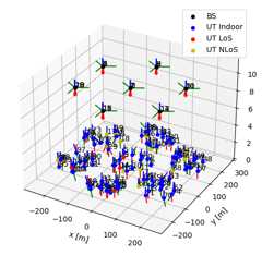
# Create channel modelchannel_model=UMi(carrier_frequency=carrier_frequency,o2i_model='low',# 'low' or 'high'ut_array=ut_array,bs_array=bs_array,direction='uplink',enable_pathloss=True,enable_shadow_fading=True)channel_model.set_topology(*topology)channel_model.show_topology()
Channel
Next, the channel frequency response is computed over the OFDM resource grid.
[9]:
# Set up the OFDM resource gridresource_grid=ResourceGrid(num_ofdm_symbols=num_ofdm_sym,fft_size=num_subcarriers,subcarrier_spacing=subcarrier_spacing,num_tx=num_ut_per_sector,num_streams_per_tx=num_streams_per_ut)# Instantiate the OFDM channel generatorofdm_channel=GenerateOFDMChannel(channel_model,resource_grid)# Generate the OFDM channel matrix in the uplink# [batch_size, num_rx=num_bs, num_rx_ant, num_tx=num_ut, num_tx_ant, num_ofdm_symbols, num_subcarriers]h_freq_ul=ofdm_channel(batch_size)# [batch_size, num_rx=num_ut, num_rx_ant, num_tx=num_bs, num_tx_ant, num_ofdm_symbols, num_subcarriers]h_freq_dl=tf.transpose(h_freq_ul,[0,3,4,1,2,5,6])
[10]:
# For simplicity, all users are allocated simultaneously on all resourcesis_scheduled=tf.fill([batch_size,num_bs,num_ofdm_sym,num_subcarriers,num_ut_per_sector,num_streams_per_ut],True)num_allocated_subcarriers=tf.fill([batch_size,num_bs,num_ofdm_sym,num_ut_per_sector],num_subcarriers)
Uplink power control
According to the open-loop power control procedure defined in 3GPP TS 38.213[1], the transmit power allocated to a user compensates the pathloss\(PL\) from the serving base station by a factor\(\alpha\in[0;1]\) while targeting a received power\(P_0\) [dBm]:
\(P^{\mathrm{UL}} = \min \{ P_0 + \alpha PL + 10 \log_{10}(\mathrm{\#PRB}), P^{\mathrm{max}}_{\mathrm{ut}}\} \quad \mathrm{[dBm]}\)
where\(P^{\mathrm{max}}_{\mathrm{ut}}\) [dBm] is the maximum transmit power for the terminal and\(\mathrm{\#PRB}\) is the number of physical resource blocks allocated to the user.
As a first step, we compute the pathloss for each user:
[11]:
_,pathloss_serving_cell=get_pathloss(h_freq_ul,rx_tx_association=tf.cast(rx_tx_association_ul,dtype=tf.int32))defgroup_by_bs(tensor):tensor=tf.reshape(tensor,[batch_size,num_bs,num_ut_per_sector,num_ofdm_sym])# [batch_size, num_bs, num_ofdm_symbols, num_ut_per_sector]returntf.transpose(tensor,[0,1,3,2])# Group by base station# [batch_size, num_bs, num_ut_per_sector, num_ofdm_sym]pathloss_serving_cell=group_by_bs(pathloss_serving_cell)
[12]:
@tf.function(jit_compile=True)defget_sinr_uplink(h_freq,pathloss_serving_cell,alpha,p0_dbm,ut_max_power_dbm,num_allocated_subcarriers,is_scheduled):""" Compute the uplink SINR """# Per-user uplink transmit power# [batch_size, num_bs, num_ofdm_sym, num_ut_per_sector]ul_power_per_ut=open_loop_uplink_power_control(pathloss_serving_cell,num_allocated_subcarriers,alpha=alpha,p0_dbm=p0_dbm,ut_max_power_dbm=ut_max_power_dbm)# Spread power uniformly across subcarriers# [batch_size, num_bs, num_ut_per_sector, num_streams_per_ut, num_ofdm_sym,# num_subcarriers]ul_power=spread_across_subcarriers(ul_power_per_ut,is_scheduled,num_tx=num_ut_per_sector)ul_power=tf.reshape(ul_power,[batch_size,num_ut,num_streams_per_ut,num_ofdm_sym,num_subcarriers])# Compute SINRprecoded_channel=EyePrecodedChannel(resource_grid=resource_grid,stream_management=stream_management_ul)h_eff=precoded_channel(h_freq,tx_power=ul_power)lmmse_posteq_sinr=LMMSEPostEqualizationSINR(resource_grid=resource_grid,stream_management=stream_management_ul)# [batch_size, num_ofdm_symbols, num_effective_subcarriers, num_rx, num_streams_per_rx]sinr=lmmse_posteq_sinr(h_eff,no=tf.cast(no,tf.float32),interference_whitening=True)# [batch_size, num_ofdm_symbols, num_effective_subcarriers, num_ut, num_streams_per_ut]sinr=tf.reshape(sinr,sinr.shape[:-2]+[num_ut,num_streams_per_ut])returnsinr,ul_power_per_ut
Impact of parameters on system performance
[13]:
defget_se(sinr):""" Compute the spectral efficiency """se_per_ut=tf.reduce_sum(log2(1+sinr),axis=[4])# Average across OFDM symbols and subcarriersreturntf.reduce_mean(se_per_ut,axis=[1,2])# Values of (alpha, P0) to evaluatealpha_vec=np.linspace(.5,1,50)p0_dbm_vec=np.arange(-110,-69,1)# Per-user spectral efficiency per user across (alpha, P0) valuesse_per_ut_ul_mat=np.zeros([len(p0_dbm_vec),len(alpha_vec),num_ut*batch_size])ul_power_mat=np.zeros([len(p0_dbm_vec),len(alpha_vec),num_ut*batch_size])# Compute the spectral efficiency for each (alpha, P0) pairforidx_p0,p0_dbminenumerate(p0_dbm_vec):foridx_alpha,alphainenumerate(alpha_vec):# Compute SINR and UL power distribution# sinr: [batch_size, num_ofdm_symbols, num_effective_subcarriers, num_ut,# num_streams_per_ut]# ul_power_per_ut: # [batch_size, num_bs, num_ofdm_sym, num_ut_per_sector]sinr,ul_power_per_ut=get_sinr_uplink(h_freq_ul,pathloss_serving_cell,alpha,p0_dbm,ut_max_power_dbm,num_allocated_subcarriers,is_scheduled)# Compute the spectral efficiencyse_per_ut_ul_mat[idx_p0,idx_alpha,:]=get_se(sinr).numpy().flatten()# Power allocationul_power_mat[idx_p0,idx_alpha,:]=ul_power_per_ut.numpy().mean(axis=2).flatten()
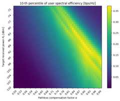
To illustrate the impact of the design parameters\((\alpha, P_0)\) on network performance, we evaluate the\(x\)-th percentile of the spectral efficiency distribution across users, that we want to maximize as a function of\((\alpha, P_0)\).
[14]:
xth_percentile=10metric_mat=np.zeros([len(p0_dbm_vec),len(alpha_vec)])foridx_p0,p0_dbminenumerate(p0_dbm_vec):foridx_alpha,alphainenumerate(alpha_vec):metric_mat[idx_p0,idx_alpha]=np.nanpercentile(se_per_ut_ul_mat[idx_p0,idx_alpha,:],xth_percentile)plt.figure(figsize=(8,6))plt.imshow(metric_mat,aspect='auto')plt.colorbar()plt.ylabel(r'Target received power $P_0$ [dBm]')plt.xlabel(r'Pathloss compensation factor $\alpha$')plt.title(f'{xth_percentile}-th percentile of user spectral efficiency [bps/Hz]')plt.yticks(np.arange(len(p0_dbm_vec)),p0_dbm_vec)plt.gca().invert_yaxis()show_every=3plt.xticks(np.arange(0,len(alpha_vec),show_every),[f'{alpha_vec[i]:.2f}'foriinrange(0,len(alpha_vec),show_every)],rotation=45)plt.yticks(np.arange(0,len(p0_dbm_vec),show_every),[p0_dbm_vec[i]foriinrange(0,len(p0_dbm_vec),show_every)],rotation=45)plt.show()
It is also interesting to evaluate the distribution of the power allocation across users.
[15]:
defget_cdf(values):""" Computes the Cumulative Distribution Function (CDF) of the input """values=np.array(values).flatten()n=len(values)sorted_val=np.sort(values)cumulative_prob=np.arange(1,n+1)/nreturnsorted_val,cumulative_probalpha_po_vec=[(.9,-100),(1.,-100),(.9,-80)]fig,ax=plt.subplots()foralpha,poinalpha_po_vec:idx_p0,idx_alpha=np.argmin(np.abs(p0_dbm_vec-po)),np.argmin(np.abs(alpha_vec-alpha))ax.plot(*get_cdf(ul_power_mat[idx_p0,idx_alpha,:]*1e3),label=fr'$\alpha=${alpha_vec[idx_alpha]:.2f}, $P_0$={p0_dbm_vec[idx_p0]}')ax.plot([dbm_to_watt(ut_max_power_dbm)*1e3]*2,[0,1],'k--',label='max UT power')ax.set_xlabel('Per-user uplink transmit power [mW]')ax.set_ylabel('CDF')ax.legend()ax.grid()plt.show()
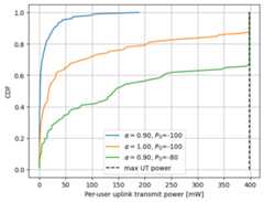
As expected, an increase of either the pathloss compensation factor\(\alpha\) or the target received power\(P_0\) leads to a higher power allocation, which eventually saturates at the maximum transmit power for the user terminal.
Downlink power control
In the downlink, the base station distributes the per-resource transmit power\(p_u\) across different users\(u=1,\dots,P\).
The functiondownlink_fair_power_control maximizes a fairness function\(g^{(f)}\) defined as in[2] of the maximum attainable throughput:
where\(q_u\) is a measure of the channel quality for user\(u\) and\(r_u\) is the number of allocated resources for\(u\).
The base station transmit power must not exceed\(P^{\mathrm{max}}_{\mathrm{bs}}\):
Moreover, to ensure that all scheduled users obtain a positive throughput, we can impose a lower bound on the individual allocated powers:
where\(0\le \rho \le 1\). Note that if\(\rho=1\), then all users obtain the same power allocation.
To estimate the channel quality for each user, we compute the pathloss from the serving cell and the interference from all neighboring cells.
[16]:
# Pathloss# [batch_size, num_ut, num_bs, num_ofdm_symbols], [batch_size, num_ut, num_ofdm_symbols]pathloss_all_pairs,pathloss_serving_cell=get_pathloss(h_freq_dl,rx_tx_association=tf.cast(rx_tx_association_dl,dtype=tf.int32))# Interference from all base stations# [batch_size, num_ut, num_ofdm_symbols]one=tf.cast(1,pathloss_serving_cell.dtype)interference_dl=tf.reduce_sum(one/pathloss_all_pairs,axis=-2)-one/pathloss_serving_cellinterference_dl*=bs_max_power# Group by base station# [batch_size, num_bs, num_ut_per_sector, num_ofdm_sym]pathloss_serving_cell=group_by_bs(pathloss_serving_cell)interference_dl=group_by_bs(interference_dl)
Impact of parameters on system performance
The downlink power allocation procedure indownlink_fair_power_control is governed by two parameters:
the fairness parameter\(f\), defined as in[2].If\(f=0\), then the sum of throughput is maximized, favoring users with good channel conditions while potentially leaving those in poor conditions without power.As\(f\) increases, the allocation becomes more egalitarian across users;
the guaranteed power ratio\(\rho\), which defines the minimum power allocation per user.
To evaluate the impact of these two design parameters on the network performance, we evaluate the spectral efficiency distribution as\((f,\rho)\) vary.
[17]:
defget_sinr_downlink(guaranteed_power_ratio,fairness_dl):""" Compute the downlink SINR """# [batch_size, num_bs, num_ofdm_symbols, num_ut_per_sector]dl_power_per_ut,_=downlink_fair_power_control(pathloss_serving_cell,interference_dl+no,num_allocated_subcarriers,bs_max_power_dbm=bs_max_power_dbm,guaranteed_power_ratio=guaranteed_power_ratio,fairness=fairness_dl)# Spread power uniformly across subcarriers# [batch_size, num_bs, num_ut_per_sector, num_streams_per_ut, num_ofdm_sym, num_subcarriers]dl_power=spread_across_subcarriers(dl_power_per_ut,is_scheduled,num_tx=1)dl_power=tf.reshape(dl_power,[batch_size,num_bs,num_streams_per_bs,num_ofdm_sym,num_subcarriers])precoded_channel=RZFPrecodedChannel(resource_grid=resource_grid,stream_management=stream_management_dl)h_eff=precoded_channel(h_freq_dl,tx_power=dl_power,alpha=no)lmmse_posteq_sinr=LMMSEPostEqualizationSINR(resource_grid=resource_grid,stream_management=stream_management_dl)# [batch_size, num_ofdm_symbols, num_subcarriers, num_ut, num_streams_per_ut]sinr=lmmse_posteq_sinr(h_eff,no=no,interference_whitening=True)returnsinr,dl_power_per_ut
[18]:
# Fairness parameters to evaluatefairness_dl_vec=[0,.5,1]# Guaranteed power ratio to evaluateguaranteed_power_ratio_vec=[0,.3]# Per-user spectral efficiency per user across (fairness, guaranteed power ratio) valuesse_per_ut_dl_mat=np.zeros([len(fairness_dl_vec),len(guaranteed_power_ratio_vec),num_ut*batch_size])dl_power_mat=np.zeros([len(fairness_dl_vec),len(guaranteed_power_ratio_vec),num_ut*batch_size])# Compute the spectral efficiency for each (fairness, guaranteed power ratio) pairforidx_guar,guaranteed_power_ratioinenumerate(guaranteed_power_ratio_vec):foridx_fair,fairness_dlinenumerate(fairness_dl_vec):# Compute SINR and DL power distributionsinr,dl_power_per_ut=get_sinr_downlink(guaranteed_power_ratio,fairness_dl)# Spectral efficiencyse_per_ut_dl_mat[idx_fair,idx_guar,:]=get_se(sinr).numpy().flatten()# Power allocationdl_power_mat[idx_fair,idx_guar,:]=dl_power_per_ut.numpy().mean(axis=2).flatten()
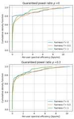
Finally, we visualize the spectral efficiency distribution across the different values of fairness\(f\) and guaranteed power ratio\(\rho\).
[19]:
fig,axs=plt.subplots(len(guaranteed_power_ratio_vec),figsize=(5,4*len(guaranteed_power_ratio_vec)))foridx_guar,guaranteed_power_ratioinenumerate(guaranteed_power_ratio_vec):axs[idx_guar].set_title(r'Guaranteed power ratio $\rho$ ='+f'{guaranteed_power_ratio}')foridx_fair,fairness_dlinenumerate(fairness_dl_vec):axs[idx_guar].plot(*get_cdf(se_per_ut_dl_mat[idx_fair,idx_guar,:]),label=f'Fairness $f$ ={fairness_dl}')foraxinaxs:ax.grid()ax.legend()ax.set_xlabel('Per-user spectral efficiency [bps/Hz]')ax.set_ylabel('Cumulative density function')fig.tight_layout()plt.show()
It is also interesting to evaluate the power allocation distribution for different values of fairness\(f\) and guaranteed power ratio\(\rho\).
[20]:
fairness_guar_ratio_vec=[(0,0),(0,.5),(1,0)]fig,ax=plt.subplots()forfairness,guaranteed_power_ratioinfairness_guar_ratio_vec:idx_fair=np.argmin(np.abs(np.array(fairness_dl_vec)-fairness))idx_guar=np.argmin(np.abs(np.array(guaranteed_power_ratio_vec)-guaranteed_power_ratio))ax.plot(*get_cdf(dl_power_mat[idx_fair,idx_guar,:]),label=fr'$f$={fairness_dl_vec[idx_fair]:.1f}, $\rho$={guaranteed_power_ratio_vec[idx_guar]:.1f}')ax.plot([dbm_to_watt(bs_max_power_dbm)]*2,[0,1],'k--',label='max BS power')ax.set_xlabel('Per-user downlink transmit power [W]')ax.set_ylabel('Cumulative density function')ax.legend()ax.grid()plt.show()
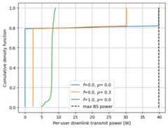
For computational efficiency, we recommend setting\(f=0\) and choosing\(\rho >0\) to ensure that all users receive some power allocation.
Conclusions
Power allocation in both uplink and downlink requires a global perspective on the network to ensure fairness across all served users.
We provide two built-in functions for this purpose:
open_loop_uplink_power_control for uplink power allocation following the open-loop procedure described in 3GPP TS 38.213[1]
downlink_fair_power_control for fair downlink power allocation.