Weighted Belief Propagation Decoding
This notebooks implements theWeighted Belief Propagation (BP) algorithm as proposed by Nachmaniet al. in [1]. The main idea is to leverage BP decoding by additional trainable weights that scale each outgoing variable node (VN) and check node (CN) message. These weights provide additional degrees of freedom and can be trained by stochastic gradient descent (SGD) to improve the BP performance for the given code. If all weights are initialized with1, the algorithm equals theclassical BPalgorithm and, thus, the concept can be seen as a generalized BP decoder.
Our main focus is to show how Sionna can lower the barrier-to-entry for state-of-the-art research. For this, you will investigate:
How to implement the multi-loss BP decoding with Sionna
How a single scaling factor can lead to similar results
What happens for training of the 5G LDPC code
The setup includes the following components:
LDPC BP Decoder
Gaussian LLR source
Please note that we implement a simplified version of the original algorithm consisting of two major simplifications:
) Only outgoing variable node (VN) messages are weighted. This is possible as the VN operation is linear and it would only increase the memory complexity without increasing theexpressive power of the neural network.
) We use the same shared weights for all iterations. This can potentially influence the final performance, however, simplifies the implementation and allows to run the decoder with different number of iterations.
Note: If you are not familiar with all-zero codeword-based simulations please have a look into theBit-Interleaved Coded Modulation example notebook first.
Table of Contents
GPU Configuration and Imports
[1]:
importosifos.getenv("CUDA_VISIBLE_DEVICES")isNone:gpu_num=0# Use "" to use the CPUos.environ["CUDA_VISIBLE_DEVICES"]=f"{gpu_num}"os.environ['TF_CPP_MIN_LOG_LEVEL']='3'# Import Sionnatry:importsionna.phyexceptImportErrorase:importsysif'google.colab'insys.modules:# Install Sionna in Google Colabprint("Installing Sionna and restarting the runtime. Please run the cell again.")os.system("pip install sionna")os.kill(os.getpid(),5)else:raiseeimporttensorflowastf# Configure the notebook to use only a single GPU and allocate only as much memory as needed# For more details, see https://www.tensorflow.org/guide/gpugpus=tf.config.list_physical_devices('GPU')ifgpus:try:tf.config.experimental.set_memory_growth(gpus[0],True)exceptRuntimeErrorase:print(e)# Avoid warnings from TensorFlowtf.get_logger().setLevel('ERROR')sionna.phy.config.seed=42# Set seed for reproducible random number generation# Import required Sionna componentsfromsionna.phy.fec.ldpcimportLDPCBPDecoder,LDPC5GEncoder,LDPC5GDecoder,WeightedBPCallbackfromsionna.phy.fec.utilsimportGaussianPriorSource,load_parity_check_examples,llr2mifromsionna.phy.utilsimportebnodb2no,hard_decisionsfromsionna.phy.utils.metricsimportcompute_berfromsionna.phy.utils.plottingimportPlotBERfromtensorflow.keras.lossesimportBinaryCrossentropyfromsionna.phyimportBlock%matplotlib inlineimportmatplotlib.pyplotaspltimportnumpyasnp
Weighted BP for BCH Codes
First, we define the trainable model consisting of:
LDPC BP decoder
Gaussian LLR source
The idea of the multi-loss function in [1] is to average the loss overall iterations, i.e., not just the final estimate is evaluated. This requires to call the BP decoderiteration-wise by settingnum_iter=1 andreturn_state=True such that the decoder will perform a single iteration and returns its current estimate while also providing the internal messages for the next iteration.
A few comments:
We assume the transmission of the all-zero codeword. This allows to train and analyze the decoder without the need of an encoder. Remark: The final decoder can be used for arbitrary codewords.
We directly generate the channel LLRs with
GaussianPriorSource. The equivalent LLR distribution could be achieved by transmitting the all-zero codeword over an AWGN channel with BPSK modulation.For the proposedmulti-loss [1] (i.e., the loss is averaged over all iterations), we need to access the decoders intermediate output after each iteration. This is done by calling the decoding function multiple times while setting
return_stateto True, i.e., the decoder continuous the decoding process at the last message state.
The BP decoder itself does not have any trainable weights. However, the LDPCBPDecoder API allows to register custom callback functions after each VN/CN node update step. In this tutorial, we use theWeightedBPCallback to apply trainable weights to each exchanged internal decoder message. Similarly, offset-corrected BP can be made trainable.
[ ]:
classWeightedBP(Block):"""System model for BER simulations of weighted BP decoding. This model uses `GaussianPriorSource` to mimic the LLRs after demapping of QPSK symbols transmitted over an AWGN channel. Parameters ---------- pcm: ndarray The parity-check matrix of the code under investigation. num_iter: int Number of BP decoding iterations. Input ----- batch_size: int or tf.int The batch_size used for the simulation. ebno_db: float or tf.float A float defining the simulation SNR. Output ------ (u, u_hat, loss): Tuple: u: tf.float32 A tensor of shape `[batch_size, k] of 0s and 1s containing the transmitted information bits. u_hat: tf.float32 A tensor of shape `[batch_size, k] of 0s and 1s containing the estimated information bits. loss: tf.float32 Binary cross-entropy loss between `u` and `u_hat`. """def__init__(self,pcm,num_iter=5):super().__init__()# add trainable weights via decoder callbacksself.edge_weights=WeightedBPCallback(num_edges=np.sum(pcm))# init componentsself.decoder=LDPCBPDecoder(pcm,num_iter=1,# iterations are done via outer loop (to access intermediate results for multi-loss)return_state=True,# decoder stores internal messages after callhard_out=False,# we need to access soft-informationcn_update="boxplus",v2c_callbacks=[self.edge_weights])# register callback to make the decoder trainable# used to generate llrs during training (see example notebook on all-zero codeword trick)self.llr_source=GaussianPriorSource()self._num_iter=num_iterself._bce=BinaryCrossentropy(from_logits=True)defcall(self,batch_size,ebno_db):noise_var=ebnodb2no(ebno_db,num_bits_per_symbol=2,# QPSKcoderate=self.decoder.coderate)# all-zero CW to calculate loss / BERc=tf.zeros([batch_size,self.decoder.n])# Gaussian LLR sourcellr=self.llr_source([batch_size,self.decoder.n],noise_var)# --- implement multi-loss as proposed by Nachmani et al. [1]---loss=0msg_v2c=None# internal state of decoderforiinrange(self._num_iter):c_hat,msg_v2c=self.decoder(llr,msg_v2c=msg_v2c)# perform one decoding iteration; decoder returns soft-valuesloss+=self._bce(c,c_hat)# add loss after each iterationloss/=self._num_iter# scale loss by number of iterationsreturnc,c_hat,loss
Load a parity-check matrix used for the experiment. We use the same BCH(63,45) code as in [1]. The code can be replaced by any parity-check matrix of your choice.
[3]:
pcm_id=1# (63,45) BCH code parity check matrixpcm,k,n,coderate=load_parity_check_examples(pcm_id=pcm_id,verbose=True)num_iter=10# set number of decoding iterations# and initialize the modelmodel=WeightedBP(pcm=pcm,num_iter=num_iter)
n: 63, k: 45, coderate: 0.714
Note: weighted BP tends to work better for small number of iterations. The effective gains (compared to the baseline with same number of iterations) vanish with more iterations.
Weightsbefore Training and Simulation of BER
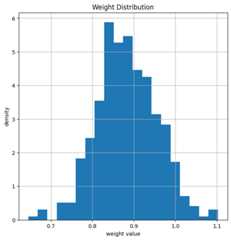
Let us plot the weights after initialization of the decoder to verify that everything is properly initialized. This is equivalent theclassical BP decoder.
[4]:
# count number of weights/edgesprint("Total number of weights: ",np.size(model.edge_weights.weights))# and show the weight distributionmodel.edge_weights.show_weights()
Total number of weights: 432

We first simulate (and store) the BER performancebefore training. For this, we use thePlotBER class, which provides a convenient way to store the results for later comparison.
[5]:
# SNR to simulate the resultsebno_dbs=np.array(np.arange(1,7,0.5))mc_iters=100# number of Monte Carlo iterations# we generate a new PlotBER() object to simulate, store and plot the BER resultsber_plot=PlotBER("Weighted BP")# simulate and plot the BER curve of the untrained decoderber_plot.simulate(model,ebno_dbs=ebno_dbs,batch_size=1000,num_target_bit_errors=2000,# stop sim after 2000 bit errorslegend="Untrained",soft_estimates=True,max_mc_iter=mc_iters,forward_keyboard_interrupt=False,graph_mode="graph");
EbNo [dB] | BER | BLER | bit errors | num bits | block errors | num blocks | runtime [s] | status--------------------------------------------------------------------------------------------------------------------------------------- 1.0 | 8.6508e-02 | 9.6500e-01 | 5450 | 63000 | 965 | 1000 | 6.6 |reached target bit errors 1.5 | 7.4159e-02 | 9.2100e-01 | 4672 | 63000 | 921 | 1000 | 0.0 |reached target bit errors 2.0 | 5.9968e-02 | 8.0400e-01 | 3778 | 63000 | 804 | 1000 | 0.0 |reached target bit errors 2.5 | 4.6937e-02 | 6.8300e-01 | 2957 | 63000 | 683 | 1000 | 0.0 |reached target bit errors 3.0 | 3.2381e-02 | 4.8800e-01 | 2040 | 63000 | 488 | 1000 | 0.0 |reached target bit errors 3.5 | 2.1563e-02 | 3.5450e-01 | 2717 | 126000 | 709 | 2000 | 0.1 |reached target bit errors 4.0 | 1.3878e-02 | 2.4100e-01 | 2623 | 189000 | 723 | 3000 | 0.1 |reached target bit errors 4.5 | 8.2103e-03 | 1.4550e-01 | 2069 | 252000 | 582 | 4000 | 0.1 |reached target bit errors 5.0 | 3.8342e-03 | 7.3222e-02 | 2174 | 567000 | 659 | 9000 | 0.3 |reached target bit errors 5.5 | 2.3333e-03 | 4.3643e-02 | 2058 | 882000 | 611 | 14000 | 0.5 |reached target bit errors 6.0 | 1.0389e-03 | 1.9677e-02 | 2029 | 1953000 | 610 | 31000 | 1.1 |reached target bit errors 6.5 | 4.5465e-04 | 9.2714e-03 | 2005 | 4410000 | 649 | 70000 | 2.5 |reached target bit errors

Training
We now train the model for a fixed number of SGD training iterations.
Note: this is a very basic implementation of the training loop. You can also try more sophisticated training loops with early stopping, different hyper-parameters or optimizers etc.
[6]:
# training parametersbatch_size=1000train_iter=200ebno_db=4.0clip_value_grad=10# gradient clipping for stable training convergence# try also different optimizers or different hyperparametersoptimizer=tf.keras.optimizers.Adam(learning_rate=1e-2)@tf.functiondeftrain_step():withtf.GradientTape()astape:b,llr,loss=model(batch_size,ebno_db)grads=tape.gradient(loss,tape.watched_variables())grads=[tf.clip_by_value(g,-clip_value_grad,clip_value_grad,name=None)forgingrads]optimizer.apply_gradients(zip(grads,tape.watched_variables()))returnloss,b,llrforitinrange(0,train_iter):loss,b,llr=train_step()# calculate and print intermediate metrics# only for information# this has no impact on the trainingifit%10==0: # evaluate every 10 iterations# calculate ber from received LLRsb_hat=hard_decisions(llr)# hard decided LLRs firstber=compute_ber(b,b_hat)# and print resultsmi=llr2mi(llr,-2*b+1).numpy()# calculate bit-wise mutual informationl=loss.numpy()# copy loss to numpy for printingprint(f"Current loss:{l:3f} ber:{ber:.4f} bmi:{mi:.3f}".format())
Current loss: 0.049836 ber: 0.0132 bmi: 0.939Current loss: 0.050902 ber: 0.0129 bmi: 0.943Current loss: 0.047043 ber: 0.0129 bmi: 0.945Current loss: 0.041731 ber: 0.0117 bmi: 0.948Current loss: 0.043182 ber: 0.0131 bmi: 0.948Current loss: 0.037416 ber: 0.0116 bmi: 0.955Current loss: 0.039514 ber: 0.0126 bmi: 0.951Current loss: 0.038904 ber: 0.0123 bmi: 0.949Current loss: 0.038560 ber: 0.0118 bmi: 0.951Current loss: 0.043944 ber: 0.0137 bmi: 0.944Current loss: 0.039379 ber: 0.0124 bmi: 0.950Current loss: 0.040292 ber: 0.0136 bmi: 0.948Current loss: 0.040030 ber: 0.0132 bmi: 0.950Current loss: 0.039854 ber: 0.0124 bmi: 0.950Current loss: 0.039948 ber: 0.0132 bmi: 0.951Current loss: 0.038435 ber: 0.0119 bmi: 0.956Current loss: 0.042012 ber: 0.0128 bmi: 0.949Current loss: 0.042593 ber: 0.0127 bmi: 0.947Current loss: 0.043055 ber: 0.0137 bmi: 0.946Current loss: 0.036739 ber: 0.0121 bmi: 0.954
Results
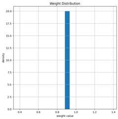
After training, the weights of the decoder have changed. In average, the weights are smaller after training.
[7]:
model.edge_weights.show_weights()# show weights AFTER training
And let us compare the new BER performance. For this, we can simply call the ber_plot.simulate() function again as it internally stores all previous results (ifadd_results is True).
[8]:
ebno_dbs=np.array(np.arange(1,7,0.5))batch_size=10000mc_ites=100ber_plot.simulate(model,ebno_dbs=ebno_dbs,batch_size=1000,num_target_bit_errors=2000,# stop sim after 2000 bit errorslegend="Trained",max_mc_iter=mc_iters,soft_estimates=True,graph_mode="graph");
EbNo [dB] | BER | BLER | bit errors | num bits | block errors | num blocks | runtime [s] | status--------------------------------------------------------------------------------------------------------------------------------------- 1.0 | 8.9317e-02 | 9.9500e-01 | 5627 | 63000 | 995 | 1000 | 3.2 |reached target bit errors 1.5 | 7.7492e-02 | 9.8000e-01 | 4882 | 63000 | 980 | 1000 | 0.0 |reached target bit errors 2.0 | 6.3794e-02 | 9.3400e-01 | 4019 | 63000 | 934 | 1000 | 0.0 |reached target bit errors 2.5 | 5.0635e-02 | 8.3500e-01 | 3190 | 63000 | 835 | 1000 | 0.0 |reached target bit errors 3.0 | 3.3794e-02 | 6.0000e-01 | 2129 | 63000 | 600 | 1000 | 0.0 |reached target bit errors 3.5 | 2.1627e-02 | 4.1150e-01 | 2725 | 126000 | 823 | 2000 | 0.1 |reached target bit errors 4.0 | 1.2545e-02 | 2.5067e-01 | 2371 | 189000 | 752 | 3000 | 0.1 |reached target bit errors 4.5 | 6.2275e-03 | 1.2900e-01 | 2354 | 378000 | 774 | 6000 | 0.2 |reached target bit errors 5.0 | 3.1921e-03 | 6.7100e-02 | 2011 | 630000 | 671 | 10000 | 0.4 |reached target bit errors 5.5 | 1.2540e-03 | 2.9500e-02 | 2054 | 1638000 | 767 | 26000 | 0.9 |reached target bit errors 6.0 | 4.7642e-04 | 1.2662e-02 | 2041 | 4284000 | 861 | 68000 | 2.4 |reached target bit errors 6.5 | 2.1810e-04 | 5.8800e-03 | 1374 | 6300000 | 588 | 100000 | 3.6 |reached max iterations

Further Experiments
You will now see that the memory footprint can be drastically reduced by using the same weight for all messages. In the second part we will apply the concept to the 5G LDPC codes.
Damped BP
It is well-known that scaling of LLRs / messages can help to improve the performance of BP decoding in some scenarios [3,4]. In particular, this works well for very short codes such as the code we are currently analyzing.
We now follow the basic idea of [2] and scale all weights with the same scalar.
[9]:
# get weights of trained modelweights_bp=model.edge_weights.weights# calc mean value of weightsdamping_factor=tf.reduce_mean(weights_bp)# set all weights to the SAME constant scalingweights_damped=tf.ones_like(weights_bp)*damping_factor# and apply the new weightsmodel.edge_weights.weights.assign(weights_damped)# let us have look at the new weights againmodel.edge_weights.show_weights()# and simulate the BER againleg_str=f"Damped BP (scaling factor{damping_factor.numpy():.3f})"ber_plot.simulate(model,ebno_dbs=ebno_dbs,batch_size=1000,num_target_bit_errors=2000,# stop sim after 2000 bit errorslegend=leg_str,max_mc_iter=mc_iters,soft_estimates=True,graph_mode="graph");
EbNo [dB] | BER | BLER | bit errors | num bits | block errors | num blocks | runtime [s] | status--------------------------------------------------------------------------------------------------------------------------------------- 1.0 | 8.8540e-02 | 9.9400e-01 | 5578 | 63000 | 994 | 1000 | 3.2 |reached target bit errors 1.5 | 7.6889e-02 | 9.7700e-01 | 4844 | 63000 | 977 | 1000 | 0.0 |reached target bit errors 2.0 | 6.2968e-02 | 9.3200e-01 | 3967 | 63000 | 932 | 1000 | 0.0 |reached target bit errors 2.5 | 4.7063e-02 | 7.7600e-01 | 2965 | 63000 | 776 | 1000 | 0.0 |reached target bit errors 3.0 | 3.4413e-02 | 6.1400e-01 | 2168 | 63000 | 614 | 1000 | 0.0 |reached target bit errors 3.5 | 2.2960e-02 | 4.1950e-01 | 2893 | 126000 | 839 | 2000 | 0.1 |reached target bit errors 4.0 | 1.2392e-02 | 2.4133e-01 | 2342 | 189000 | 724 | 3000 | 0.1 |reached target bit errors 4.5 | 5.8862e-03 | 1.2183e-01 | 2225 | 378000 | 731 | 6000 | 0.2 |reached target bit errors 5.0 | 2.8320e-03 | 6.0333e-02 | 2141 | 756000 | 724 | 12000 | 0.4 |reached target bit errors 5.5 | 1.2990e-03 | 2.9760e-02 | 2046 | 1575000 | 744 | 25000 | 0.9 |reached target bit errors 6.0 | 5.1146e-04 | 1.3111e-02 | 2030 | 3969000 | 826 | 63000 | 2.2 |reached target bit errors 6.5 | 2.2333e-04 | 6.1000e-03 | 1407 | 6300000 | 610 | 100000 | 3.5 |reached max iterations

When looking at the results, we observe almost the same performance although we only scale by a single scalar. This implies that the number of weights of our model is by far too large and the memory footprint could be reduced significantly. However, isn’t it fascinating to see that this simple concept of weighted BP leads to the same results as the concept ofdamped BP?
Note: for more iterations it could be beneficial to implement an individual damping per iteration.
Learning the 5G LDPC Code
In this Section, you will experience what happens if we apply the same concept to the 5G LDPC code (including rate matching).
For this, we need to define a new model.
[ ]:
classWeightedBP5G(Block):"""System model for BER simulations of weighted BP decoding for 5G LDPC codes. This model uses `GaussianPriorSource` to mimic the LLRs after demapping of QPSK symbols transmitted over an AWGN channel. Parameters ---------- k: int Number of information bits per codeword. n: int Codeword length. num_iter: int Number of BP decoding iterations. Input ----- batch_size: int or tf.int The batch_size used for the simulation. ebno_db: float or tf.float A float defining the simulation SNR. Output ------ (u, u_hat, loss): Tuple: u: tf.float32 A tensor of shape `[batch_size, k] of 0s and 1s containing the transmitted information bits. u_hat: tf.float32 A tensor of shape `[batch_size, k] of 0s and 1s containing the estimated information bits. loss: tf.float32 Binary cross-entropy loss between `u` and `u_hat`. """def__init__(self,k,n,num_iter=20):super().__init__()# we need to initialize an encoder for the 5G parametersself.encoder=LDPC5GEncoder(k,n)# add trainable weights via decoder callbacksself.edge_weights=WeightedBPCallback(num_edges=int(np.sum(self.encoder.pcm)))self.decoder=LDPC5GDecoder(self.encoder,num_iter=1,# iterations are done via outer loop (to access intermediate results for multi-loss)return_state=True,hard_out=False,prune_pcm=False,cn_update="boxplus",v2c_callbacks=[self.edge_weights,])# register callbackself.llr_source=GaussianPriorSource()self._num_iter=num_iterself._coderate=k/nself._bce=BinaryCrossentropy(from_logits=True)defcall(self,batch_size,ebno_db):noise_var=ebnodb2no(ebno_db,num_bits_per_symbol=2,# QPSKcoderate=self._coderate)# BPSK modulated all-zero CWc=tf.zeros([batch_size,k])# decoder only returns info bits# use fake llrs from GA# works as BP is symmetricllr=self.llr_source([batch_size,n],noise_var)# --- implement multi-loss is proposed by Nachmani et al. ---loss=0msg_v2c=Noneforiinrange(self._num_iter):c_hat,msg_v2c=self.decoder(llr,msg_v2c=msg_v2c)# perform one decoding iteration; decoder returns soft-valuesloss+=self._bce(c,c_hat)# add loss after each iterationreturnc,c_hat,loss
[11]:
# generate modelnum_iter=10k=400n=800model5G=WeightedBP5G(k,n,num_iter=num_iter)# generate baseline BERebno_dbs=np.array(np.arange(0,4,0.25))mc_iters=100# number of monte carlo iterationsber_plot_5G=PlotBER("Weighted BP for 5G LDPC")# simulate the untrained performanceber_plot_5G.simulate(model5G,ebno_dbs=ebno_dbs,batch_size=1000,num_target_bit_errors=2000,# stop sim after 2000 bit errorslegend="Untrained",soft_estimates=True,max_mc_iter=mc_iters,graph_mode="graph");
EbNo [dB] | BER | BLER | bit errors | num bits | block errors | num blocks | runtime [s] | status--------------------------------------------------------------------------------------------------------------------------------------- 0.0 | 1.6887e-01 | 1.0000e+00 | 67548 | 400000 | 1000 | 1000 | 3.9 |reached target bit errors 0.25 | 1.4882e-01 | 1.0000e+00 | 59528 | 400000 | 1000 | 1000 | 0.1 |reached target bit errors 0.5 | 1.2150e-01 | 9.9800e-01 | 48600 | 400000 | 998 | 1000 | 0.1 |reached target bit errors 0.75 | 9.7977e-02 | 9.8300e-01 | 39191 | 400000 | 983 | 1000 | 0.1 |reached target bit errors 1.0 | 6.5448e-02 | 9.3500e-01 | 26179 | 400000 | 935 | 1000 | 0.1 |reached target bit errors 1.25 | 4.2583e-02 | 8.2000e-01 | 17033 | 400000 | 820 | 1000 | 0.1 |reached target bit errors 1.5 | 2.2090e-02 | 6.3100e-01 | 8836 | 400000 | 631 | 1000 | 0.1 |reached target bit errors 1.75 | 9.1425e-03 | 3.7800e-01 | 3657 | 400000 | 378 | 1000 | 0.1 |reached target bit errors 2.0 | 2.7050e-03 | 1.7850e-01 | 2164 | 800000 | 357 | 2000 | 0.2 |reached target bit errors 2.25 | 8.3750e-04 | 7.1000e-02 | 2010 | 2400000 | 426 | 6000 | 0.5 |reached target bit errors 2.5 | 2.3580e-04 | 2.1773e-02 | 2075 | 8800000 | 479 | 22000 | 2.0 |reached target bit errors 2.75 | 3.7100e-05 | 5.0700e-03 | 1484 | 40000000 | 507 | 100000 | 8.8 |reached max iterations 3.0 | 3.9750e-06 | 8.7000e-04 | 159 | 40000000 | 87 | 100000 | 8.9 |reached max iterations 3.25 | 5.2500e-07 | 1.4000e-04 | 21 | 40000000 | 14 | 100000 | 8.9 |reached max iterations 3.5 | 3.0000e-07 | 5.0000e-05 | 12 | 40000000 | 5 | 100000 | 8.8 |reached max iterations 3.75 | 0.0000e+00 | 0.0000e+00 | 0 | 40000000 | 0 | 100000 | 8.8 |reached max iterationsSimulation stopped as no error occurred @ EbNo = 3.8 dB.

And let’s train this new model.
[12]:
# training parametersbatch_size=1000train_iter=200clip_value_grad=10# gradient clipping seems to be important# smaller training SNR as the new code is longer (=stronger) than beforeebno_db=1.5# rule of thumb: train at ber = 1e-2# try also different optimizers or different hyperparametersoptimizer=tf.keras.optimizers.Adam(learning_rate=1e-2)@tf.functiondeftrain_step():withtf.GradientTape()astape:b,llr,loss=model5G(batch_size,ebno_db)grads=tape.gradient(loss,tape.watched_variables())grads=[tf.clip_by_value(g,-clip_value_grad,clip_value_grad,name=None)forgingrads]optimizer.apply_gradients(zip(grads,tape.watched_variables()))returnloss,b,llr# and let's goforitinrange(0,train_iter):loss,b,llr=train_step()# calculate and print intermediate metricsifit%10==0:# calculate berb_hat=hard_decisions(llr)ber=compute_ber(b,b_hat)# and print resultsmi=llr2mi(llr,-2*b+1).numpy()# calculate bit-wise mutual informationl=loss.numpy()print(f"Current loss:{l:3f} ber:{ber:.4f} bmi:{mi:.3f}".format())
Current loss: 1.717313 ber: 0.0215 bmi: 0.921Current loss: 1.717737 ber: 0.0208 bmi: 0.924Current loss: 1.692114 ber: 0.0204 bmi: 0.925Current loss: 1.733131 ber: 0.0220 bmi: 0.919Current loss: 1.733311 ber: 0.0219 bmi: 0.920Current loss: 1.708051 ber: 0.0205 bmi: 0.924Current loss: 1.730341 ber: 0.0222 bmi: 0.918Current loss: 1.738736 ber: 0.0218 bmi: 0.919Current loss: 1.713310 ber: 0.0206 bmi: 0.923Current loss: 1.708243 ber: 0.0213 bmi: 0.923Current loss: 1.683718 ber: 0.0202 bmi: 0.925Current loss: 1.704449 ber: 0.0206 bmi: 0.923Current loss: 1.730718 ber: 0.0215 bmi: 0.921Current loss: 1.704801 ber: 0.0209 bmi: 0.924Current loss: 1.716135 ber: 0.0216 bmi: 0.921Current loss: 1.744884 ber: 0.0224 bmi: 0.918Current loss: 1.722892 ber: 0.0213 bmi: 0.922Current loss: 1.711179 ber: 0.0209 bmi: 0.923Current loss: 1.711154 ber: 0.0215 bmi: 0.921Current loss: 1.732857 ber: 0.0212 bmi: 0.921
We now simulate the new results and compare it to the untrained results.
[13]:
ebno_dbs=np.array(np.arange(0,4,0.25))batch_size=1000mc_iters=100ber_plot_5G.simulate(model5G,ebno_dbs=ebno_dbs,batch_size=batch_size,num_target_bit_errors=2000,# stop sim after 2000 bit errorslegend="Trained",max_mc_iter=mc_iters,soft_estimates=True,graph_mode="graph");
EbNo [dB] | BER | BLER | bit errors | num bits | block errors | num blocks | runtime [s] | status--------------------------------------------------------------------------------------------------------------------------------------- 0.0 | 1.6552e-01 | 1.0000e+00 | 66207 | 400000 | 1000 | 1000 | 3.6 |reached target bit errors 0.25 | 1.4709e-01 | 1.0000e+00 | 58835 | 400000 | 1000 | 1000 | 0.1 |reached target bit errors 0.5 | 1.2446e-01 | 1.0000e+00 | 49785 | 400000 | 1000 | 1000 | 0.1 |reached target bit errors 0.75 | 9.4812e-02 | 9.8600e-01 | 37925 | 400000 | 986 | 1000 | 0.1 |reached target bit errors 1.0 | 6.7075e-02 | 9.3900e-01 | 26830 | 400000 | 939 | 1000 | 0.1 |reached target bit errors 1.25 | 4.3540e-02 | 8.4200e-01 | 17416 | 400000 | 842 | 1000 | 0.1 |reached target bit errors 1.5 | 2.3047e-02 | 6.4500e-01 | 9219 | 400000 | 645 | 1000 | 0.1 |reached target bit errors 1.75 | 9.4325e-03 | 3.8600e-01 | 3773 | 400000 | 386 | 1000 | 0.1 |reached target bit errors 2.0 | 2.9487e-03 | 1.6850e-01 | 2359 | 800000 | 337 | 2000 | 0.2 |reached target bit errors 2.25 | 7.8071e-04 | 6.4857e-02 | 2186 | 2800000 | 454 | 7000 | 0.6 |reached target bit errors 2.5 | 1.6767e-04 | 1.9033e-02 | 2012 | 12000000 | 571 | 30000 | 2.7 |reached target bit errors 2.75 | 3.2150e-05 | 4.5300e-03 | 1286 | 40000000 | 453 | 100000 | 8.8 |reached max iterations 3.0 | 5.9500e-06 | 8.4000e-04 | 238 | 40000000 | 84 | 100000 | 8.8 |reached max iterations 3.25 | 6.2500e-07 | 1.4000e-04 | 25 | 40000000 | 14 | 100000 | 8.8 |reached max iterations 3.5 | 2.2500e-07 | 5.0000e-05 | 9 | 40000000 | 5 | 100000 | 8.8 |reached max iterations 3.75 | 1.0000e-07 | 1.0000e-05 | 4 | 40000000 | 1 | 100000 | 8.8 |reached max iterations
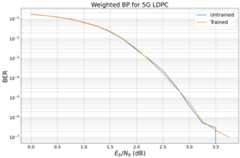
Unfortunately, we observe only very minor gains for the 5G LDPC code. We empirically observed that gain vanishes for more iterations and longer codewords, i.e., for most practical use-cases of the 5G LDPC code the gains are only minor.
However, there may be othercodesongraphs that benefit from the principle idea of weighted BP - or other channel setups? Feel free to adjust this notebook and train for your favorite code / channel.
Other ideas for own experiments:
Implement weighted BP with unique weights per iteration.
Apply the concept to (scaled) min-sum decoding as in [5].
Can you replace the complete CN update by a neural network?
Verify the results from all-zero simulations for areal system simulation with explicit encoder and random data
What happens in combination with higher order modulation?
References
[1] E. Nachmani, Y. Be’ery and D. Burshtein, “Learning to Decode Linear Codes Using Deep Learning,” IEEE Annual Allerton Conference on Communication, Control, and Computing (Allerton), pp. 341-346., 2016.https://arxiv.org/pdf/1607.04793.pdf
[2] M. Lian, C. Häger, and H. Pfister, “What can machine learning teach us about communications?” IEEE Information Theory Workshop (ITW), pp. 1-5. 2018.
[3] ] M. Pretti, “A message passing algorithm with damping,” J. Statist. Mech.: Theory Practice, p. 11008, Nov. 2005.
[4] J.S. Yedidia, W.T. Freeman and Y. Weiss, “Constructing free energy approximations and Generalized Belief Propagation algorithms,” IEEE Transactions on Information Theory, 2005.
[5] E. Nachmani, E. Marciano, L. Lugosch, W. Gross, D. Burshtein and Y. Be’ery, “Deep learning methods for improved decoding of linear codes,” IEEE Journal of Selected Topics in Signal Processing, vol. 12, no. 1, pp.119-131, 2018.