

Note
Go to the endto download the full example code.
Annotations#
Annotations are graphical elements, often pieces of text, that explain, addcontext to, or otherwise highlight some portion of the visualized data.annotate supports a number of coordinate systems for flexiblypositioning data and annotations relative to each other and a variety ofoptions of for styling the text. Axes.annotate also provides an optional arrowfrom the text to the data and this arrow can be styled in various ways.text can also be used for simple text annotation, but does notprovide as much flexibility in positioning and styling asannotate.
Artist instance
Basic annotation#
In an annotation, there are two points to consider: the location of the databeing annotatedxy and the location of the annotation textxytext. Bothof these arguments are(x,y) tuples:
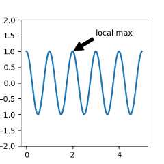
In this example, both thexy (arrow tip) andxytext locations(text location) are in data coordinates. There are a variety of othercoordinate systems one can choose -- you can specify the coordinatesystem ofxy andxytext with one of the following strings forxycoords andtextcoords (default is 'data')
argument | coordinate system |
|---|---|
'figure points' | points from the lower left corner of the figure |
'figure pixels' | pixels from the lower left corner of the figure |
'figure fraction' | (0, 0) is lower left of figure and (1, 1) is upper right |
'axes points' | points from lower left corner of the Axes |
'axes pixels' | pixels from lower left corner of the Axes |
'axes fraction' | (0, 0) is lower left of Axes and (1, 1) is upper right |
'data' | use the axes data coordinate system |
The following strings are also valid arguments fortextcoords
argument | coordinate system |
|---|---|
'offset points' | offset (in points) from the xy value |
'offset pixels' | offset (in pixels) from the xy value |
For physical coordinate systems (points or pixels) the origin is thebottom-left of the figure or Axes. Points aretypographic pointsmeaning that they are a physical unit measuring 1/72 of an inch. Points andpixels are discussed in further detail inPlotting in physical coordinates.
Annotating data#
This example places the text coordinates in fractional axes coordinates:

Annotating an Artist#
Annotations can be positioned relative to anArtist instance by passingthat Artist in asxycoords. Thenxy is interpreted as a fraction of theArtist's bounding box.
importmatplotlib.patchesasmpatchesfig,ax=plt.subplots(figsize=(3,3))arr=mpatches.FancyArrowPatch((1.25,1.5),(1.75,1.5),arrowstyle='->,head_width=.15',mutation_scale=20)ax.add_patch(arr)ax.annotate("label",(.5,.5),xycoords=arr,ha='center',va='bottom')ax.set(xlim=(1,2),ylim=(1,2))

Here the annotation is placed at position (.5,.5) relative to the arrow'slower left corner and is vertically and horizontally at that position.Vertically, the bottom aligns to that reference point so that the labelis above the line. For an example of chaining annotation Artists, see theArtist section ofCoordinate systems for annotations.
Annotating with arrows#
You can enable drawing of an arrow from the text to the annotated pointby giving a dictionary of arrow properties in the optional keywordargumentarrowprops.
arrowprops key | description |
|---|---|
width | the width of the arrow in points |
frac | the fraction of the arrow length occupied by the head |
headwidth | the width of the base of the arrow head in points |
shrink | move the tip and base some percent away fromthe annotated point and text |
**kwargs | any key for |
In the example below, thexy point is in the data coordinate systemsincexycoords defaults to 'data'. For a polar Axes, this is in(theta, radius) space. The text in this example is placed in thefractional figure coordinate system.matplotlib.text.Textkeyword arguments likehorizontalalignment,verticalalignment andfontsize are passed fromannotate to theText instance.
fig=plt.figure()ax=fig.add_subplot(projection='polar')r=np.arange(0,1,0.001)theta=2*2*np.pi*rline,=ax.plot(theta,r,color='#ee8d18',lw=3)ind=800thisr,thistheta=r[ind],theta[ind]ax.plot([thistheta],[thisr],'o')ax.annotate('a polar annotation',xy=(thistheta,thisr),# theta, radiusxytext=(0.05,0.05),# fraction, fractiontextcoords='figure fraction',arrowprops=dict(facecolor='black',shrink=0.05),horizontalalignment='left',verticalalignment='bottom')

For more on plotting with arrows, seeCustomizing annotation arrows
Placing text annotations relative to data#
Annotations can be positioned at a relative offset to thexy input toannotation by setting thetextcoords keyword argument to'offsetpoints'or'offsetpixels'.
fig,ax=plt.subplots(figsize=(3,3))x=[1,3,5,7,9]y=[2,4,6,8,10]annotations=["A","B","C","D","E"]ax.scatter(x,y,s=20)forxi,yi,textinzip(x,y,annotations):ax.annotate(text,xy=(xi,yi),xycoords='data',xytext=(1.5,1.5),textcoords='offset points')

The annotations are offset 1.5 points (1.5*1/72 inches) from thexy values.
Advanced annotation#
We recommend readingBasic annotation,text()andannotate() before reading this section.
Annotating with boxed text#
text takes abbox keyword argument, which draws a box around thetext:
fig,ax=plt.subplots(figsize=(5,5))t=ax.text(0.5,0.5,"Direction",ha="center",va="center",rotation=45,size=15,bbox=dict(boxstyle="rarrow,pad=0.3",fc="lightblue",ec="steelblue",lw=2))
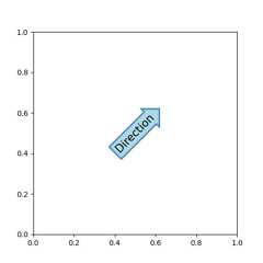
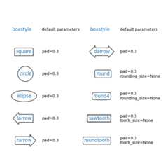
The arguments are the name of the box style with its attributes askeyword arguments. Currently, following box styles are implemented:
Class | Name | Attrs |
|---|---|---|
Circle |
| pad=0.3 |
DArrow |
| pad=0.3 |
Ellipse |
| pad=0.3 |
LArrow |
| pad=0.3 |
RArrow |
| pad=0.3 |
Round |
| pad=0.3,rounding_size=None |
Round4 |
| pad=0.3,rounding_size=None |
Roundtooth |
| pad=0.3,tooth_size=None |
Sawtooth |
| pad=0.3,tooth_size=None |
Square |
| pad=0.3 |
The patch object (box) associated with the text can be accessed using:
bb=t.get_bbox_patch()
The return value is aFancyBboxPatch; patch properties(facecolor, edgewidth, etc.) can be accessed and modified as usual.FancyBboxPatch.set_boxstyle sets the box shape:
bb.set_boxstyle("rarrow",pad=0.6)
The attribute arguments can also be specified within the stylename with separating comma:
bb.set_boxstyle("rarrow, pad=0.6")
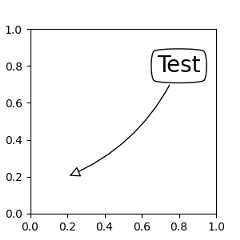
Defining custom box styles#
Custom box styles can be implemented as a function that takes arguments specifyingboth a rectangular box and the amount of "mutation", and returns the "mutated" path.The specific signature is the one ofcustom_box_style below.
Here, we return a new path which adds an "arrow" shape on the left of the box.
The custom box style can then be used by passingbbox=dict(boxstyle=custom_box_style,...) toAxes.text.
frommatplotlib.pathimportPathdefcustom_box_style(x0,y0,width,height,mutation_size):""" Given the location and size of the box, return the path of the box around it. Rotation is automatically taken care of. Parameters ---------- x0, y0, width, height : float Box location and size. mutation_size : float Mutation reference scale, typically the text font size. """# paddingmypad=0.3pad=mutation_size*mypad# width and height with padding added.width=width+2*padheight=height+2*pad# boundary of the padded boxx0,y0=x0-pad,y0-padx1,y1=x0+width,y0+height# return the new pathreturnPath([(x0,y0),(x1,y0),(x1,y1),(x0,y1),(x0-pad,(y0+y1)/2),(x0,y0),(x0,y0)],closed=True)fig,ax=plt.subplots(figsize=(3,3))ax.text(0.5,0.5,"Test",size=30,va="center",ha="center",rotation=30,bbox=dict(boxstyle=custom_box_style,alpha=0.2))

Likewise, custom box styles can be implemented as classes that implement__call__.
The classes can then be registered into theBoxStyle._style_list dict,which allows specifying the box style as a string,bbox=dict(boxstyle="registered_name,param=value,...",...).Note that this registration relies on internal APIs and is therefore notofficially supported.
frommatplotlib.patchesimportBoxStyleclassMyStyle:"""A simple box."""def__init__(self,pad=0.3):""" The arguments must be floats and have default values. Parameters ---------- pad : float amount of padding """self.pad=padsuper().__init__()def__call__(self,x0,y0,width,height,mutation_size):""" Given the location and size of the box, return the path of the box around it. Rotation is automatically taken care of. Parameters ---------- x0, y0, width, height : float Box location and size. mutation_size : float Reference scale for the mutation, typically the text font size. """# paddingpad=mutation_size*self.pad# width and height with padding addedwidth=width+2*padheight=height+2*pad# boundary of the padded boxx0,y0=x0-pad,y0-padx1,y1=x0+width,y0+height# return the new pathreturnPath([(x0,y0),(x1,y0),(x1,y1),(x0,y1),(x0-pad,(y0+y1)/2),(x0,y0),(x0,y0)],closed=True)BoxStyle._style_list["angled"]=MyStyle# Register the custom style.fig,ax=plt.subplots(figsize=(3,3))ax.text(0.5,0.5,"Test",size=30,va="center",ha="center",rotation=30,bbox=dict(boxstyle="angled,pad=0.5",alpha=0.2))delBoxStyle._style_list["angled"]# Unregister it.

Similarly, you can define a customConnectionStyle and a customArrowStyle. Viewthe source code atpatches to learn how each class is defined.
Customizing annotation arrows#
An arrow connectingxy toxytext can be optionally drawn byspecifying thearrowprops argument. To draw only an arrow, useempty string as the first argument:
fig,ax=plt.subplots(figsize=(3,3))ax.annotate("",xy=(0.2,0.2),xycoords='data',xytext=(0.8,0.8),textcoords='data',arrowprops=dict(arrowstyle="->",connectionstyle="arc3"))

The arrow is drawn as follows:
A path connecting the two points is created, as specified by theconnectionstyle parameter.
The path is clipped to avoid patchespatchA andpatchB, if these areset.
The path is further shrunk byshrinkA andshrinkB (in pixels).
The path is transmuted to an arrow patch, as specified by thearrowstyleparameter.

The creation of the connecting path between two points is controlled byconnectionstyle key and the following styles are available:
Name | Attrs |
|---|---|
| angleA=90,angleB=0,rad=0.0 |
| angleA=90,angleB=0 |
| angleA=0,angleB=0,armA=None,armB=None,rad=0.0 |
| rad=0.0 |
| armA=0.0,armB=0.0,fraction=0.3,angle=None |
Note that "3" inangle3 andarc3 is meant to indicate that theresulting path is a quadratic spline segment (three controlpoints). As will be discussed below, some arrow style options can onlybe used when the connecting path is a quadratic spline.
The behavior of each connection style is (limitedly) demonstrated in theexample below. (Warning: The behavior of thebar style is currently notwell-defined and may be changed in the future).

Connection styles for annotations
The connecting path (after clipping and shrinking) is then mutated toan arrow patch, according to the givenarrowstyle:
Name | Attrs |
|---|---|
| None |
| head_length=0.4,head_width=0.2 |
| widthB=1.0,lengthB=0.2,angleB=None |
| widthA=1.0,widthB=1.0 |
| head_length=0.4,head_width=0.2 |
| head_length=0.4,head_width=0.2 |
| head_length=0.4,head_width=0.2 |
| head_length=0.4,head_width=0.2 |
| head_length=0.4,head_width=0.2 |
| head_length=0.4,head_width=0.4,tail_width=0.4 |
| head_length=0.5,head_width=0.5,tail_width=0.2 |
| tail_width=0.3,shrink_factor=0.5 |

Some arrowstyles only work with connection styles that generate aquadratic-spline segment. They arefancy,simple, andwedge.For these arrow styles, you must use the "angle3" or "arc3" connectionstyle.
If the annotation string is given, the patch is set to the bbox patchof the text by default.
fig,ax=plt.subplots(figsize=(3,3))ax.annotate("Test",xy=(0.2,0.2),xycoords='data',xytext=(0.8,0.8),textcoords='data',size=20,va="center",ha="center",arrowprops=dict(arrowstyle="simple",connectionstyle="arc3,rad=-0.2"))

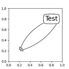
As withtext, a box around the text can be drawn using thebboxargument.
fig,ax=plt.subplots(figsize=(3,3))ann=ax.annotate("Test",xy=(0.2,0.2),xycoords='data',xytext=(0.8,0.8),textcoords='data',size=20,va="center",ha="center",bbox=dict(boxstyle="round4",fc="w"),arrowprops=dict(arrowstyle="-|>",connectionstyle="arc3,rad=-0.2",fc="w"))
By default, the starting point is set to the center of the textextent. This can be adjusted withrelpos key value. The valuesare normalized to the extent of the text. For example, (0, 0) meanslower-left corner and (1, 1) means top-right.
fig,ax=plt.subplots(figsize=(3,3))ann=ax.annotate("Test",xy=(0.2,0.2),xycoords='data',xytext=(0.8,0.8),textcoords='data',size=20,va="center",ha="center",bbox=dict(boxstyle="round4",fc="w"),arrowprops=dict(arrowstyle="-|>",connectionstyle="arc3,rad=0.2",relpos=(0.,0.),fc="w"))ann=ax.annotate("Test",xy=(0.2,0.2),xycoords='data',xytext=(0.8,0.8),textcoords='data',size=20,va="center",ha="center",bbox=dict(boxstyle="round4",fc="w"),arrowprops=dict(arrowstyle="-|>",connectionstyle="arc3,rad=-0.2",relpos=(1.,0.),fc="w"))
Placing Artist at anchored Axes locations#
There are classes of artists that can be placed at an anchoredlocation in the Axes. A common example is the legend. This typeof artist can be created by using theOffsetBox class. A fewpredefined classes are available inmatplotlib.offsetbox and inmpl_toolkits.axes_grid1.anchored_artists.
frommatplotlib.offsetboximportAnchoredTextfig,ax=plt.subplots(figsize=(3,3))at=AnchoredText("Figure 1a",prop=dict(size=15),frameon=True,loc='upper left')at.patch.set_boxstyle("round,pad=0.,rounding_size=0.2")ax.add_artist(at)

Theloc keyword has same meaning as in the legend command.
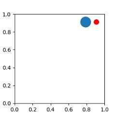
A simple application is when the size of the artist (or collection ofartists) is known in pixel size during the time of creation. Forexample, If you want to draw a circle with fixed size of 20 pixel x 20pixel (radius = 10 pixel), you can utilizeAnchoredDrawingArea. The instanceis created with a size of the drawing area (in pixels), and arbitrary artistscan be added to the drawing area. Note that the extents of the artists that areadded to the drawing area are not related to the placement of the drawingarea itself. Only the initial size matters.
The artists that are added to the drawing area should not have atransform set (it will be overridden) and the dimensions of thoseartists are interpreted as a pixel coordinate, i.e., the radius of thecircles in above example are 10 pixels and 5 pixels, respectively.
frommatplotlib.patchesimportCirclefrommpl_toolkits.axes_grid1.anchored_artistsimportAnchoredDrawingAreafig,ax=plt.subplots(figsize=(3,3))ada=AnchoredDrawingArea(40,20,0,0,loc='upper right',pad=0.,frameon=False)p1=Circle((10,10),10)ada.drawing_area.add_artist(p1)p2=Circle((30,10),5,fc="r")ada.drawing_area.add_artist(p2)ax.add_artist(ada)
Sometimes, you want your artists to scale with the data coordinate (orcoordinates other than canvas pixels). You can useAnchoredAuxTransformBox class.This is similar toAnchoredDrawingArea except thatthe extent of the artist is determined during the drawing time respecting thespecified transform.
The ellipse in the example below will have width and heightcorresponding to 0.1 and 0.4 in data coordinates and will beautomatically scaled when the view limits of the Axes change.
frommatplotlib.patchesimportEllipsefrommpl_toolkits.axes_grid1.anchored_artistsimportAnchoredAuxTransformBoxfig,ax=plt.subplots(figsize=(3,3))box=AnchoredAuxTransformBox(ax.transData,loc='upper left')el=Ellipse((0,0),width=0.1,height=0.4,angle=30)# in data coordinates!box.drawing_area.add_artist(el)ax.add_artist(box)

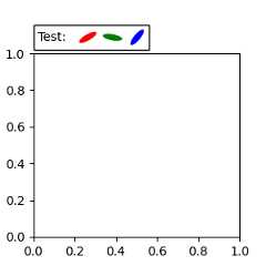
Another method of anchoring an artist relative to a parent Axes or anchorpoint is via thebbox_to_anchor argument ofAnchoredOffsetbox. Thisartist can then be automatically positioned relative to another artist usingHPacker andVPacker:
frommatplotlib.offsetboximport(AnchoredOffsetbox,DrawingArea,HPacker,TextArea)fig,ax=plt.subplots(figsize=(3,3))box1=TextArea(" Test: ",textprops=dict(color="k"))box2=DrawingArea(60,20,0,0)el1=Ellipse((10,10),width=16,height=5,angle=30,fc="r")el2=Ellipse((30,10),width=16,height=5,angle=170,fc="g")el3=Ellipse((50,10),width=16,height=5,angle=230,fc="b")box2.add_artist(el1)box2.add_artist(el2)box2.add_artist(el3)box=HPacker(children=[box1,box2],align="center",pad=0,sep=5)anchored_box=AnchoredOffsetbox(loc='lower left',child=box,pad=0.,frameon=True,bbox_to_anchor=(0.,1.02),bbox_transform=ax.transAxes,borderpad=0.,)ax.add_artist(anchored_box)fig.subplots_adjust(top=0.8)
Note that, unlike inLegend, thebbox_transform is set toIdentityTransform by default
Coordinate systems for annotations#
Matplotlib Annotations support several types of coordinate systems. Theexamples inBasic annotation used thedata coordinate system;Some others more advanced options are:
Transform instance#
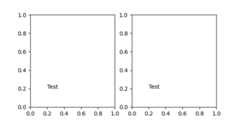
Transforms map coordinates into different coordinate systems, usually thedisplay coordinate system. SeeTransformations Tutorial for a detailedexplanation. Here Transform objects are used to identify the coordinatesystem of the corresponding points. For example, theAxes.transAxestransform positions the annotation relative to the Axes coordinates; thereforeusing it is identical to setting the coordinate system to "axes fraction":
fig,(ax1,ax2)=plt.subplots(nrows=1,ncols=2,figsize=(6,3))ax1.annotate("Test",xy=(0.2,0.2),xycoords=ax1.transAxes)ax2.annotate("Test",xy=(0.2,0.2),xycoords="axes fraction")
Another commonly usedTransform instance isAxes.transData. Thistransform is the coordinate system of the data plotted in the Axes. In thisexample, it is used to draw an arrow between related data points in twoAxes. We have passed an empty text because in this case, the annotationconnects data points.
x=np.linspace(-1,1)fig,(ax1,ax2)=plt.subplots(nrows=1,ncols=2,figsize=(6,3))ax1.plot(x,-x**3)ax2.plot(x,-3*x**2)ax2.annotate("",xy=(0,0),xycoords=ax1.transData,xytext=(0,0),textcoords=ax2.transData,arrowprops=dict(arrowstyle="<->"))

Artist instance#
Thexy value (orxytext) is interpreted as a fractional coordinate of thebounding box (bbox) of the artist:
fig,ax=plt.subplots(nrows=1,ncols=1,figsize=(3,3))an1=ax.annotate("Test 1",xy=(0.5,0.5),xycoords="data",va="center",ha="center",bbox=dict(boxstyle="round",fc="w"))an2=ax.annotate("Test 2",xy=(1,0.5),xycoords=an1,# (1, 0.5) of an1's bboxxytext=(30,0),textcoords="offset points",va="center",ha="left",bbox=dict(boxstyle="round",fc="w"),arrowprops=dict(arrowstyle="->"))
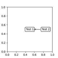
Note that you must ensure that the extent of the coordinate artist (an1 inthis example) is determined beforean2 gets drawn. Usually, this meansthatan2 needs to be drawn afteran1. The base class for all boundingboxes isBboxBase
Callable that returnsTransform ofBboxBase#
A callable object that takes the renderer instance as single argument, andreturns either aTransform or aBboxBase. For example, the returnvalue ofArtist.get_window_extent is a bbox, so this method is identicalto (2) passing in the artist:
fig,ax=plt.subplots(nrows=1,ncols=1,figsize=(3,3))an1=ax.annotate("Test 1",xy=(0.5,0.5),xycoords="data",va="center",ha="center",bbox=dict(boxstyle="round",fc="w"))an2=ax.annotate("Test 2",xy=(1,0.5),xycoords=an1.get_window_extent,xytext=(30,0),textcoords="offset points",va="center",ha="left",bbox=dict(boxstyle="round",fc="w"),arrowprops=dict(arrowstyle="->"))

Artist.get_window_extent is the bounding box of the Axes object and istherefore identical to setting the coordinate system to axes fraction:
fig,(ax1,ax2)=plt.subplots(nrows=1,ncols=2,figsize=(6,3))an1=ax1.annotate("Test1",xy=(0.5,0.5),xycoords="axes fraction")an2=ax2.annotate("Test 2",xy=(0.5,0.5),xycoords=ax2.get_window_extent)

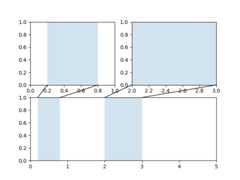
Blended coordinate specification#
A blended pair of coordinate specifications -- the first for thex-coordinate, and the second is for the y-coordinate. For example, x=0.5 isin data coordinates, and y=1 is in normalized axes coordinates:
fig,ax=plt.subplots(figsize=(3,3))ax.annotate("Test",xy=(0.5,1),xycoords=("data","axes fraction"))ax.axvline(x=.5,color='lightgray')ax.set(xlim=(0,2),ylim=(1,2))

Any of the supported coordinate systems can be used in a blendedspecification. For example, the text "Anchored to 1 & 2" is positionedrelative to the twoText Artists:

text.OffsetFrom#
Sometimes, you want your annotation with some "offset points", not from theannotated point but from some other point or artist.text.OffsetFrom isa helper for such cases.
frommatplotlib.textimportOffsetFromfig,ax=plt.subplots(figsize=(3,3))an1=ax.annotate("Test 1",xy=(0.5,0.5),xycoords="data",va="center",ha="center",bbox=dict(boxstyle="round",fc="w"))offset_from=OffsetFrom(an1,(0.5,0))an2=ax.annotate("Test 2",xy=(0.1,0.1),xycoords="data",xytext=(0,-10),textcoords=offset_from,# xytext is offset points from "xy=(0.5, 0), xycoords=an1"va="top",ha="center",bbox=dict(boxstyle="round",fc="w"),arrowprops=dict(arrowstyle="->"))

Non-text annotations#
Using ConnectionPatch#
ConnectionPatch is like an annotation without text. Whileannotateis sufficient in most situations,ConnectionPatch is useful when you wantto connect points in different Axes. For example, here we connect the pointxy in the data coordinates ofax1 to pointxy in the data coordinatesofax2:
frommatplotlib.patchesimportConnectionPatchfig,(ax1,ax2)=plt.subplots(nrows=1,ncols=2,figsize=(6,3))xy=(0.3,0.2)con=ConnectionPatch(xyA=xy,coordsA=ax1.transData,xyB=xy,coordsB=ax2.transData)fig.add_artist(con)

Here, we added theConnectionPatch to thefigure(withadd_artist) rather than to either Axes. This ensures thatthe ConnectionPatch artist is drawn on top of both Axes, and is also necessarywhen usingconstrained_layoutfor positioning the Axes.
Zoom effect between Axes#
mpl_toolkits.axes_grid1.inset_locator defines some patch classes useful forinterconnecting two Axes.
The code for this figure is atAxes zoom effect andfamiliarity withTransformations Tutorialis recommended.
Total running time of the script: (0 minutes 4.953 seconds)