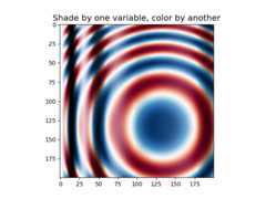
importmatplotlib.pyplotaspltimportnumpyasnpfrommatplotlib.colorsimportLightSource,Normalizedefdisplay_colorbar():"""Display a correct numeric colorbar for a shaded plot."""y,x=np.mgrid[-4:2:200j,-4:2:200j]z=10*np.cos(x**2+y**2)cmap=plt.colormaps["copper"]ls=LightSource(315,45)rgb=ls.shade(z,cmap)fig,ax=plt.subplots()ax.imshow(rgb,interpolation='bilinear')# Use a proxy artist for the colorbar...im=ax.imshow(z,cmap=cmap)im.remove()fig.colorbar(im,ax=ax)ax.set_title('Using a colorbar with a shaded plot',size='x-large')defavoid_outliers():"""Use a custom norm to control the displayed z-range of a shaded plot."""y,x=np.mgrid[-4:2:200j,-4:2:200j]z=10*np.cos(x**2+y**2)# Add some outliers...z[100,105]=2000z[120,110]=-9000ls=LightSource(315,45)fig,(ax1,ax2)=plt.subplots(ncols=2,figsize=(8,4.5))rgb=ls.shade(z,plt.colormaps["copper"])ax1.imshow(rgb,interpolation='bilinear')ax1.set_title('Full range of data')rgb=ls.shade(z,plt.colormaps["copper"],vmin=-10,vmax=10)ax2.imshow(rgb,interpolation='bilinear')ax2.set_title('Manually set range')fig.suptitle('Avoiding Outliers in Shaded Plots',size='x-large')defshade_other_data():"""Demonstrates displaying different variables through shade and color."""y,x=np.mgrid[-4:2:200j,-4:2:200j]z1=np.sin(x**2)# Data to hillshadez2=np.cos(x**2+y**2)# Data to colornorm=Normalize(z2.min(),z2.max())cmap=plt.colormaps["RdBu"]ls=LightSource(315,45)rgb=ls.shade_rgb(cmap(norm(z2)),z1)fig,ax=plt.subplots()ax.imshow(rgb,interpolation='bilinear')ax.set_title('Shade by one variable, color by another',size='x-large')display_colorbar()avoid_outliers()shade_other_data()plt.show()

DownloadJupyternotebook:advanced_hillshading.ipynb

DownloadPythonsourcecode:advanced_hillshading.py

Downloadzipped:advanced_hillshading.zip