

Note
Go to the endto download the full example code.
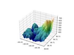
Custom hillshading in a 3D surface plot#
Demonstrates using custom hillshading in a 3D surface plot.
importmatplotlib.pyplotaspltimportnumpyasnpfrommatplotlibimportcbookfrommatplotlib.colorsimportLightSource# Load and format datadem=cbook.get_sample_data('jacksboro_fault_dem.npz')z=dem['elevation']nrows,ncols=z.shapex=np.linspace(dem['xmin'],dem['xmax'],ncols)y=np.linspace(dem['ymin'],dem['ymax'],nrows)x,y=np.meshgrid(x,y)region=np.s_[5:50,5:50]x,y,z=x[region],y[region],z[region]# Set up plotfig,ax=plt.subplots(subplot_kw=dict(projection='3d'))ls=LightSource(270,45)# To use a custom hillshading mode, override the built-in shading and pass# in the rgb colors of the shaded surface calculated from "shade".rgb=ls.shade(z,cmap=plt.colormaps["gist_earth"],vert_exag=0.1,blend_mode='soft')surf=ax.plot_surface(x,y,z,rstride=1,cstride=1,facecolors=rgb,linewidth=0,antialiased=False,shade=False)plt.show()
Tags:plot-type: 3Dlevel: intermediatedomain: cartography