

Note
Go to the endto download the full example code.
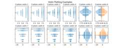
Violin plot basics#
Violin plots are similar to histograms and box plots in that they showan abstract representation of the probability distribution of thesample. Rather than showing counts of data points that fall into binsor order statistics, violin plots use kernel density estimation (KDE) tocompute an empirical distribution of the sample. That computationis controlled by several parameters. This example demonstrates how tomodify the number of points at which the KDE is evaluated (points)and how to modify the bandwidth of the KDE (bw_method).
For more information on violin plots and KDE, the scikit-learn docshave a great section:https://scikit-learn.org/stable/modules/density.html
importmatplotlib.pyplotaspltimportnumpyasnp# Fixing random state for reproducibilitynp.random.seed(19680801)# fake datafs=10# fontsizepos=[1,2,4,5,7,8]data=[np.random.normal(0,std,size=100)forstdinpos]fig,axs=plt.subplots(nrows=2,ncols=6,figsize=(10,4))axs[0,0].violinplot(data,pos,points=20,widths=0.3,showmeans=True,showextrema=True,showmedians=True)axs[0,0].set_title('Custom violin 1',fontsize=fs)axs[0,1].violinplot(data,pos,points=40,widths=0.5,showmeans=True,showextrema=True,showmedians=True,bw_method='silverman')axs[0,1].set_title('Custom violin 2',fontsize=fs)axs[0,2].violinplot(data,pos,points=60,widths=0.7,showmeans=True,showextrema=True,showmedians=True,bw_method=0.5)axs[0,2].set_title('Custom violin 3',fontsize=fs)axs[0,3].violinplot(data,pos,points=60,widths=0.7,showmeans=True,showextrema=True,showmedians=True,bw_method=0.5,quantiles=[[0.1],[],[],[0.175,0.954],[0.75],[0.25]])axs[0,3].set_title('Custom violin 4',fontsize=fs)axs[0,4].violinplot(data[-1:],pos[-1:],points=60,widths=0.7,showmeans=True,showextrema=True,showmedians=True,quantiles=[0.05,0.1,0.8,0.9],bw_method=0.5)axs[0,4].set_title('Custom violin 5',fontsize=fs)axs[0,5].violinplot(data[-1:],pos[-1:],points=60,widths=0.7,showmeans=True,showextrema=True,showmedians=True,quantiles=[0.05,0.1,0.8,0.9],bw_method=0.5,side='low')axs[0,5].violinplot(data[-1:],pos[-1:],points=60,widths=0.7,showmeans=True,showextrema=True,showmedians=True,quantiles=[0.05,0.1,0.8,0.9],bw_method=0.5,side='high')axs[0,5].set_title('Custom violin 6',fontsize=fs)axs[1,0].violinplot(data,pos,points=80,orientation='horizontal',widths=0.7,showmeans=True,showextrema=True,showmedians=True)axs[1,0].set_title('Custom violin 7',fontsize=fs)axs[1,1].violinplot(data,pos,points=100,orientation='horizontal',widths=0.9,showmeans=True,showextrema=True,showmedians=True,bw_method='silverman')axs[1,1].set_title('Custom violin 8',fontsize=fs)axs[1,2].violinplot(data,pos,points=200,orientation='horizontal',widths=1.1,showmeans=True,showextrema=True,showmedians=True,bw_method=0.5)axs[1,2].set_title('Custom violin 9',fontsize=fs)axs[1,3].violinplot(data,pos,points=200,orientation='horizontal',widths=1.1,showmeans=True,showextrema=True,showmedians=True,quantiles=[[0.1],[],[],[0.175,0.954],[0.75],[0.25]],bw_method=0.5)axs[1,3].set_title('Custom violin 10',fontsize=fs)axs[1,4].violinplot(data[-1:],pos[-1:],points=200,orientation='horizontal',widths=1.1,showmeans=True,showextrema=True,showmedians=True,quantiles=[0.05,0.1,0.8,0.9],bw_method=0.5)axs[1,4].set_title('Custom violin 11',fontsize=fs)axs[1,5].violinplot(data[-1:],pos[-1:],points=200,orientation='horizontal',widths=1.1,showmeans=True,showextrema=True,showmedians=True,quantiles=[0.05,0.1,0.8,0.9],bw_method=0.5,side='low')axs[1,5].violinplot(data[-1:],pos[-1:],points=200,orientation='horizontal',widths=1.1,showmeans=True,showextrema=True,showmedians=True,quantiles=[0.05,0.1,0.8,0.9],bw_method=0.5,side='high')axs[1,5].set_title('Custom violin 12',fontsize=fs)foraxinaxs.flat:ax.set_yticklabels([])fig.suptitle("Violin Plotting Examples")fig.subplots_adjust(hspace=0.4)plt.show()
Tags:plot-type: violindomain: statistics
References
The use of the following functions, methods, classes and modules is shownin this example:
Total running time of the script: (0 minutes 1.250 seconds)