Create grid-shaped combinations of Axes#

subplots

The primary function used to create figures and a grid of Axes. Itcreates and places all Axes on the figure at once, and returns anobject array with handles for the Axes in the grid. SeeFigure.subplots.

or

subplot_mosaic

A simple way to create figures and a grid of Axes, with the addedflexibility that Axes can also span rows or columns. The Axes are returnedin a labelled dictionary instead of an array. See alsoFigure.subplot_mosaic andComplex and semantic figure composition (subplot_mosaic).

Sometimes it is natural to have more than one distinct group of Axes grids,in which case Matplotlib has the concept ofSubFigure:

SubFigure

A virtual figure within a figure.

Underlying tools#

Underlying these are the concept of aGridSpec andaSubplotSpec:

GridSpec

Specifies the geometry of the grid that a subplot will beplaced. The number of rows and number of columns of the gridneed to be set. Optionally, the subplot layout parameters(e.g., left, right, etc.) can be tuned.

SubplotSpec

Specifies the location of the subplot in the givenGridSpec.

Adding single Axes at a time#

The above functions create all Axes in a single function call. It is alsopossible to add Axes one at a time, and this was originally how Matplotlibused to work. Doing so is generally less elegant and flexible, thoughsometimes useful for interactive work or to place an Axes in a customlocation:

add_axes

Adds a single Axes at a location specified by[left,bottom,width,height] in fractions of figure width or height.

subplot orFigure.add_subplot

Adds a single subplot on a figure, with 1-based indexing (inherited fromMatlab). Columns and rows can be spanned by specifying a range of gridcells.

subplot2grid

Similar topyplot.subplot, but uses 0-based indexing and two-d pythonslicing to choose cells.

As a simple example of manually adding an Axesax, lets add a 3 inch x 2 inchAxes to a 4 inch x 3 inch figure. Note that the location of the subplot isdefined as [left, bottom, width, height] in figure-normalized units:

importmatplotlib.pyplotaspltimportnumpyasnpw,h=4,3margin=0.5fig=plt.figure(figsize=(w,h),facecolor='lightblue')ax=fig.add_axes((margin/w,margin/h,(w-2*margin)/w,(h-2*margin)/h))

Basic 2x2 grid#

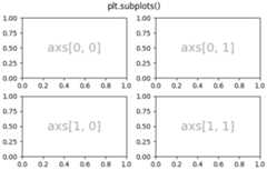
We can create a basic 2-by-2 grid of Axes usingsubplots. It returns aFigureinstance and an array ofAxes objects. The Axesobjects can be used to access methods to place artists on the Axes; herewe useannotate, but other examples could beplot,pcolormesh, etc.

fig,axs=plt.subplots(ncols=2,nrows=2,figsize=(5.5,3.5),layout="constrained")# add an artist, in this case a nice label in the middle...forrowinrange(2):forcolinrange(2):axs[row,col].annotate(f'axs[{row},{col}]',(0.5,0.5),transform=axs[row,col].transAxes,ha='center',va='center',fontsize=18,color='darkgrey')fig.suptitle('plt.subplots()')

We will annotate a lot of Axes, so let's encapsulate the annotation, ratherthan having that large piece of annotation code every time we need it:

defannotate_axes(ax,text,fontsize=18):ax.text(0.5,0.5,text,transform=ax.transAxes,ha="center",va="center",fontsize=fontsize,color="darkgrey")

The same effect can be achieved withsubplot_mosaic,but the return type is a dictionary instead of an array, where the usercan give the keys useful meanings. Here we provide two lists, each listrepresenting a row, and each element in the list a key representing thecolumn.

fig,axd=plt.subplot_mosaic([['upper left','upper right'],['lower left','lower right']],figsize=(5.5,3.5),layout="constrained")fork,axinaxd.items():annotate_axes(ax,f'axd[{k!r}]',fontsize=14)fig.suptitle('plt.subplot_mosaic()')

Grids of fixed-aspect ratio Axes#

Fixed-aspect ratio Axes are common for images or maps. However, theypresent a challenge to layout because two sets of constraints are beingimposed on the size of the Axes - that they fit in the figure and that theyhave a set aspect ratio. This leads to large gaps between Axes by default:

fig,axs=plt.subplots(2,2,layout="constrained",figsize=(5.5,3.5),facecolor='lightblue')foraxinaxs.flat:ax.set_aspect(1)fig.suptitle('Fixed aspect Axes')

One way to address this is to change the aspect of the figure to be closeto the aspect ratio of the Axes, however that requires trial and error.Matplotlib also supplieslayout="compressed", which will work withsimple grids to reduce the gaps between Axes. (Thempl_toolkits alsoprovidesImageGrid to accomplisha similar effect, but with a non-standard Axes class).

fig,axs=plt.subplots(2,2,layout="compressed",figsize=(5.5,3.5),facecolor='lightblue')foraxinaxs.flat:ax.set_aspect(1)fig.suptitle('Fixed aspect Axes: compressed')

Axes spanning rows or columns in a grid#

Sometimes we want Axes to span rows or columns of the grid.There are actually multiple ways to accomplish this, but the mostconvenient is probably to usesubplot_mosaic by repeating oneof the keys:

fig,axd=plt.subplot_mosaic([['upper left','right'],['lower left','right']],figsize=(5.5,3.5),layout="constrained")fork,axinaxd.items():annotate_axes(ax,f'axd[{k!r}]',fontsize=14)fig.suptitle('plt.subplot_mosaic()')

See below for the description of how to do the same thing usingGridSpec orsubplot2grid.

Variable widths or heights in a grid#

Bothsubplots andsubplot_mosaic allow the rowsin the grid to be different heights, and the columns to be differentwidths using thegridspec_kw keyword argument.Spacing parameters accepted byGridSpeccan be passed tosubplots andsubplot_mosaic:

gs_kw=dict(width_ratios=[1.4,1],height_ratios=[1,2])fig,axd=plt.subplot_mosaic([['upper left','right'],['lower left','right']],gridspec_kw=gs_kw,figsize=(5.5,3.5),layout="constrained")fork,axinaxd.items():annotate_axes(ax,f'axd[{k!r}]',fontsize=14)fig.suptitle('plt.subplot_mosaic()')

Nested Axes layouts#

Sometimes it is helpful to have two or more grids of Axes thatmay not need to be related to one another. The most simple way toaccomplish this is to useFigure.subfigures. Note that the subfigurelayouts are independent, so the Axes spines in each subfigure are notnecessarily aligned. See below for a more verbose way to achieve the sameeffect withGridSpecFromSubplotSpec.

fig=plt.figure(layout="constrained")subfigs=fig.subfigures(1,2,wspace=0.07,width_ratios=[1.5,1.])axs0=subfigs[0].subplots(2,2)subfigs[0].set_facecolor('lightblue')subfigs[0].suptitle('subfigs[0]\nLeft side')subfigs[0].supxlabel('xlabel for subfigs[0]')axs1=subfigs[1].subplots(3,1)subfigs[1].suptitle('subfigs[1]')subfigs[1].supylabel('ylabel for subfigs[1]')

It is also possible to nest Axes usingsubplot_mosaic usingnested lists. This method does not use subfigures, like above, so lacksthe ability to add per-subfiguresuptitle andsupxlabel, etc.Rather it is a convenience wrapper around thesubgridspecmethod described below.

inner=[['innerA'],['innerB']]outer=[['upper left',inner],['lower left','lower right']]fig,axd=plt.subplot_mosaic(outer,layout="constrained")fork,axinaxd.items():annotate_axes(ax,f'axd[{k!r}]')

Basic 2x2 grid#

We can accomplish a 2x2 grid in the same manner asplt.subplots(2,2):

fig=plt.figure(figsize=(5.5,3.5),layout="constrained")spec=fig.add_gridspec(ncols=2,nrows=2)ax0=fig.add_subplot(spec[0,0])annotate_axes(ax0,'ax0')ax1=fig.add_subplot(spec[0,1])annotate_axes(ax1,'ax1')ax2=fig.add_subplot(spec[1,0])annotate_axes(ax2,'ax2')ax3=fig.add_subplot(spec[1,1])annotate_axes(ax3,'ax3')fig.suptitle('Manually added subplots using add_gridspec')

Axes spanning rows or grids in a grid#

We can index thespec array usingNumPy slice syntaxand the new Axes will span the slice. This would be the sameasfig,axd=plt.subplot_mosaic([['ax0','ax0'],['ax1','ax2']],...):

fig=plt.figure(figsize=(5.5,3.5),layout="constrained")spec=fig.add_gridspec(2,2)ax0=fig.add_subplot(spec[0,:])annotate_axes(ax0,'ax0')ax10=fig.add_subplot(spec[1,0])annotate_axes(ax10,'ax10')ax11=fig.add_subplot(spec[1,1])annotate_axes(ax11,'ax11')fig.suptitle('Manually added subplots, spanning a column')

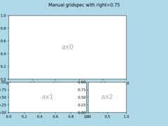
Manual adjustments to aGridSpec layout#

When aGridSpec is explicitly used, you can adjust the layoutparameters of subplots that are created from theGridSpec. Note thisoption is not compatible withconstrained layout orFigure.tight_layout which both ignoreleft andright and adjustsubplot sizes to fill the figure. Usually such manual placementrequires iterations to make the Axes tick labels not overlap the Axes.

These spacing parameters can also be passed tosubplots andsubplot_mosaic as thegridspec_kw argument.

fig=plt.figure(layout=None,facecolor='lightblue')gs=fig.add_gridspec(nrows=3,ncols=3,left=0.05,right=0.75,hspace=0.1,wspace=0.05)ax0=fig.add_subplot(gs[:-1,:])annotate_axes(ax0,'ax0')ax1=fig.add_subplot(gs[-1,:-1])annotate_axes(ax1,'ax1')ax2=fig.add_subplot(gs[-1,-1])annotate_axes(ax2,'ax2')fig.suptitle('Manual gridspec with right=0.75')

Nested layouts with SubplotSpec#

You can create nested layout similar tosubfigures usingsubgridspec. Here the Axes spinesarealigned.

Note this is also available from the more verbosegridspec.GridSpecFromSubplotSpec.

fig=plt.figure(layout="constrained")gs0=fig.add_gridspec(1,2)gs00=gs0[0].subgridspec(2,2)gs01=gs0[1].subgridspec(3,1)forainrange(2):forbinrange(2):ax=fig.add_subplot(gs00[a,b])annotate_axes(ax,f'axLeft[{a},{b}]',fontsize=10)ifa==1andb==1:ax.set_xlabel('xlabel')forainrange(3):ax=fig.add_subplot(gs01[a])annotate_axes(ax,f'axRight[{a},{b}]')ifa==2:ax.set_ylabel('ylabel')fig.suptitle('nested gridspecs')

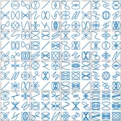
Here's a more sophisticated example of nestedGridSpec: We create an outer4x4 grid with each cell containing an inner 3x3 grid of Axes. We outlinethe outer 4x4 grid by hiding appropriate spines in each of the inner 3x3grids.

defsquiggle_xy(a,b,c,d,i=np.arange(0.0,2*np.pi,0.05)):returnnp.sin(i*a)*np.cos(i*b),np.sin(i*c)*np.cos(i*d)fig=plt.figure(figsize=(8,8),layout='constrained')outer_grid=fig.add_gridspec(4,4,wspace=0,hspace=0)forainrange(4):forbinrange(4):# gridspec inside gridspecinner_grid=outer_grid[a,b].subgridspec(3,3,wspace=0,hspace=0)axs=inner_grid.subplots()# Create all subplots for the inner grid.for(c,d),axinnp.ndenumerate(axs):ax.plot(*squiggle_xy(a+1,b+1,c+1,d+1))ax.set(xticks=[],yticks=[])# show only the outside spinesforaxinfig.get_axes():ss=ax.get_subplotspec()ax.spines.top.set_visible(ss.is_first_row())ax.spines.bottom.set_visible(ss.is_last_row())ax.spines.left.set_visible(ss.is_first_col())ax.spines.right.set_visible(ss.is_last_col())plt.show()