Plot a confidence ellipse of a two-dimensional dataset#

This example shows how to plot a confidence ellipse of atwo-dimensional dataset, using its pearson correlation coefficient.

The approach that is used to obtain the correct geometry isexplained and proved here:

https://carstenschelp.github.io/2018/09/14/Plot_Confidence_Ellipse_001.html

The method avoids the use of an iterative eigen decomposition algorithmand makes use of the fact that a normalized covariance matrix (composed ofpearson correlation coefficients and ones) is particularly easy to handle.

importmatplotlib.pyplotaspltimportnumpyasnpfrommatplotlib.patchesimportEllipseimportmatplotlib.transformsastransforms

The plotting function itself#

This function plots the confidence ellipse of the covariance of the givenarray-like variables x and y. The ellipse is plotted into the givenAxes objectax.

The radiuses of the ellipse can be controlled by n_std which is the numberof standard deviations. The default value is 3 which makes the ellipseenclose 98.9% of the points if the data is normally distributedlike in these examples (3 standard deviations in 1-D contain 99.7%of the data, which is 98.9% of the data in 2-D).

defconfidence_ellipse(x,y,ax,n_std=3.0,facecolor='none',**kwargs):"""    Create a plot of the covariance confidence ellipse of *x* and *y*.    Parameters    ----------    x, y : array-like, shape (n, )        Input data.    ax : matplotlib.axes.Axes        The Axes object to draw the ellipse into.    n_std : float        The number of standard deviations to determine the ellipse's radiuses.    **kwargs        Forwarded to `~matplotlib.patches.Ellipse`    Returns    -------    matplotlib.patches.Ellipse    """ifx.size!=y.size:raiseValueError("x and y must be the same size")cov=np.cov(x,y)pearson=cov[0,1]/np.sqrt(cov[0,0]*cov[1,1])# Using a special case to obtain the eigenvalues of this# two-dimensional dataset.ell_radius_x=np.sqrt(1+pearson)ell_radius_y=np.sqrt(1-pearson)ellipse=Ellipse((0,0),width=ell_radius_x*2,height=ell_radius_y*2,facecolor=facecolor,**kwargs)# Calculating the standard deviation of x from# the squareroot of the variance and multiplying# with the given number of standard deviations.scale_x=np.sqrt(cov[0,0])*n_stdmean_x=np.mean(x)# calculating the standard deviation of y ...scale_y=np.sqrt(cov[1,1])*n_stdmean_y=np.mean(y)transf=transforms.Affine2D() \.rotate_deg(45) \.scale(scale_x,scale_y) \.translate(mean_x,mean_y)ellipse.set_transform(transf+ax.transData)returnax.add_patch(ellipse)

A helper function to create a correlated dataset#

Creates a random two-dimensional dataset with the specifiedtwo-dimensional mean (mu) and dimensions (scale).The correlation can be controlled by the param 'dependency',a 2x2 matrix.

defget_correlated_dataset(n,dependency,mu,scale):latent=np.random.randn(n,2)dependent=latent.dot(dependency)scaled=dependent*scalescaled_with_offset=scaled+mu# return x and y of the new, correlated datasetreturnscaled_with_offset[:,0],scaled_with_offset[:,1]

Positive, negative and weak correlation#

Note that the shape for the weak correlation (right) is an ellipse,not a circle because x and y are differently scaled.However, the fact that x and y are uncorrelated is shown bythe axes of the ellipse being aligned with the x- and y-axisof the coordinate system.

np.random.seed(0)PARAMETERS={'Positive correlation':[[0.85,0.35],[0.15,-0.65]],'Negative correlation':[[0.9,-0.4],[0.1,-0.6]],'Weak correlation':[[1,0],[0,1]],}mu=2,4scale=3,5fig,axs=plt.subplots(1,3,figsize=(9,3))forax,(title,dependency)inzip(axs,PARAMETERS.items()):x,y=get_correlated_dataset(800,dependency,mu,scale)ax.scatter(x,y,s=0.5)ax.axvline(c='grey',lw=1)ax.axhline(c='grey',lw=1)confidence_ellipse(x,y,ax,edgecolor='red')ax.scatter(mu[0],mu[1],c='red',s=3)ax.set_title(title)plt.show()

Positive correlation, Negative correlation, Weak correlation

Different number of standard deviations#

A plot with n_std = 3 (blue), 2 (purple) and 1 (red)

fig,ax_nstd=plt.subplots(figsize=(6,6))dependency_nstd=[[0.8,0.75],[-0.2,0.35]]mu=0,0scale=8,5ax_nstd.axvline(c='grey',lw=1)ax_nstd.axhline(c='grey',lw=1)x,y=get_correlated_dataset(500,dependency_nstd,mu,scale)ax_nstd.scatter(x,y,s=0.5)confidence_ellipse(x,y,ax_nstd,n_std=1,label=r'$1\sigma$',edgecolor='firebrick')confidence_ellipse(x,y,ax_nstd,n_std=2,label=r'$2\sigma$',edgecolor='fuchsia',linestyle='--')confidence_ellipse(x,y,ax_nstd,n_std=3,label=r'$3\sigma$',edgecolor='blue',linestyle=':')ax_nstd.scatter(mu[0],mu[1],c='red',s=3)ax_nstd.set_title('Different standard deviations')ax_nstd.legend()plt.show()

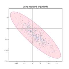
Using the keyword arguments#

Use the keyword arguments specified formatplotlib.patches.Patch in orderto have the ellipse rendered in different ways.

fig,ax_kwargs=plt.subplots(figsize=(6,6))dependency_kwargs=[[-0.8,0.5],[-0.2,0.5]]mu=2,-3scale=6,5ax_kwargs.axvline(c='grey',lw=1)ax_kwargs.axhline(c='grey',lw=1)x,y=get_correlated_dataset(500,dependency_kwargs,mu,scale)# Plot the ellipse with zorder=0 in order to demonstrate# its transparency (caused by the use of alpha).confidence_ellipse(x,y,ax_kwargs,alpha=0.5,facecolor='pink',edgecolor='purple',zorder=0)ax_kwargs.scatter(x,y,s=0.5)ax_kwargs.scatter(mu[0],mu[1],c='red',s=3)ax_kwargs.set_title('Using keyword arguments')fig.subplots_adjust(hspace=0.25)plt.show()