Repository files navigation

CEC is anRpackage that performs data points clustering using the cross–entropy clustering(CEC) method¹. This method has been developed based on information theory andcombines the speed and simplicity of k-means with the ability to use variousGaussian mixture models and automatically remove unnecessary clusters.

CEC can be installed directly fromCRAN as follows:

install.packages("CEC")

You can also use theremotes package to installthe development version ofCEC as follows:

remotes::install_github("swarm-lab/cec")

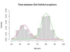
The core function of theCEC package isthecec function. In the simplest scenario, this function requires only twoarguments: an input data matrix (x) and the initial number of cluster centers(centers). For instance, here is how to identify two clusters in the waitingtimes between eruptions for the Old Faithful geyser in Yellowstone National Park,Wyoming, USA:

library("CEC")data("faithful")clusters<- cec(as.matrix(faithful[,2,drop=FALSE]),2)clusters

The functioncec returns the following important information:

• clusters$cluster: the cluster membership of each data point;
• clusters$centers: the coordinates of the centers of each cluster;
• clusters$covariances.model: the model covariance of each cluster;
• clusters$probability: the probability that a random data point belongs to agiven cluster.

Additional information concerning the number of iterations, the cost (energy)function, and the number of clusters at each iteration are also available.

You can now plot the results of the clustering process as follows:

hist(faithful$waiting,prob=TRUE,main="Time between Old Faithful eruptions",xlab="Minutes",col="lightgray",border=0,ylim= c(0,0.05))for (iin c(1:2)) {    curve(cec$probability[i]* dnorm(x,mean=cec$centers[i],sd= sqrt(cec$covariances.model[[i]][1])),add=T,col=i+1,lwd=2)  }

Like k-means, the quality of the results produced by CEC depends on the choiceof initial cluster centers. The initial locations of the centers can be chosenusing thecenters.init parameter of thecec function. It can be set to"random" to select the initial centers randomly, or to"kmeans++" to selectthem via thek-means++ method. Itis also recommended to run the clustering algorithm multiple times withdifferent cluster centers. This can easily be achieved using thenstartparameter. For instance,

clusters<- cec(as.matrix(faithful[,2,drop=FALSE]),2,method="kmeans++",nstart=10,threads=4)clusters

will run the clustering algorithm 10 times, initializing it each time with theoutput of the k-means++ algorithm. Only the best of the 10 runs (i.e. the runwith the lowest cost function) will be returned by the function.

Note that, whennstart > 1, the clustering process can be sped-up by runningit in parallel threads using thethreads parameter (more details in thepackage manual).

card.min represents the minimal cluster size, i.e. the number of points belowwhich a cluster is removed from the analysis. It can be expressed as a number ofpoints or as a percentage of the data set size.

iter.max is the maximum allowed number of iterations of the algorithm at eachstart. If the algorithm does not converge beforeiter.max is reached, thefunction will stop and return the best result so far.

One of the most important properties of the CEC algorithm is that it cancombined various Gaussian models in the same clustering process. The CEC packageincludes six Gaussian models, which can be specified via the parametertype.These models are:

type = "all"

The general Gaussian CEC algorithm gives similar results to those obtained byGaussian Mixture Models. However, the CEC does not use the EM (ExpectationMaximization) approach for minimization but a simple iteration process (Hartiganmethod). Consequently, larger data sets can be processed in shorter time.

CEC will have a tendency to divide the data into clusters in the shape ofellipses (ellipsoids in higher dimensions). For instance:

data("fourGaussians")cec<- cec(fourGaussians,centers=10,type="all",nstart=20)plot(cec,asp=1)

type = "spherical"

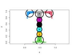
The original distribution will be approximated by spherical (radial) densities,which will result in splitting the data into disk-like clusters of arbitrarysizes (spheres in higher dimensions).

data("Tset")cec<- cec(x=Tset,centers=10,type="spherical",nstart=5)plot(cec,asp=1)

type = "fixedr"

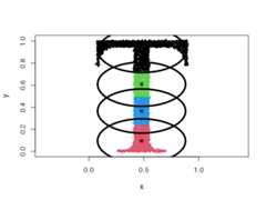
Similarly to the general spherical model, the data set will be divided intoclusters resembling disks, but with their radius determined by theparamargument.

data("Tset")cec<- cec(x=Tset,centers=10,type="fixedr",param=0.01,nstart=20)plot(cec,asp=1)

type = "diagonal"

In this case, the data will be described by ellipses for which the mainsemi-major axes are parallel to the axes of the coordinate system.

data("Tset")cec<- cec(x=Tset,centers=10,type="diagonal",nstart=5)plot(cec,asp=1)

type = "covariance"

This model clusters the data using Gaussians with a fixed covariance. Thecovariance matrix is passed to theparam argument.

data("Tset")cec<- cec(x=Tset,centers=10,card.min='10%',type="covariance",param=matrix(c(0.04,0,0,0.01),2))plot(cec,asp=1)

type = "eigenvalues"

This is similar to the previous example, but here the Gaussians have fixedeigenvalues. The eigenvalues are passed to theparam argument.

data("Tset")cec<- cec(x=Tset,centers=10,type="eigenvalues",param= c(0.01,0.001),nstart=5)plot(cec,asp=1)

type = "mean"

In this condition, the data is clustered using Gaussians with fixed mean values.The mean values of the data dimensions are passed to theparam argument.

data("Tset")cec<- cec(Tset,4,"mean",param= c(0.48,0.48),nstart=5)plot(cec,asp=1)

data("threeGaussians")cec<- cec(threeGaussians,4,"mean",param= c(0,0),nstart=10)plot(cec)

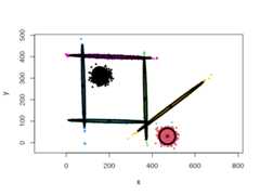
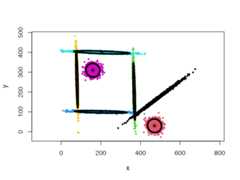
One of the most powerful properties of the CEC algorithm is the possibility ofmixing Gaussian models together. More precisely, the mixed models can bespecified by giving a list of cluster types (and a list of correspondingparameters, if needed).

data("mixShapes")cec<- cec(mixShapes,7,iter.max=3,type= c("fixedr","fixedr","eigen","eigen","eigen","eigen","eigen"),param=list(350,350, c(9000,8), c(9000,8),                  c(9000,8), c(9000,8), c(9000,8)),nstart=500,threads=10)plot(cec,asp=1)

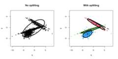
Thecec function includes an option to discover new clusters after the initialclustering has occurred. This is done by recursively trying to split eachcluster into two smaller clusters that would lower the cost function.

To enable the splitting method, thesplit argument must be set toTRUE inthecec function. For instance:

data("fourGaussians")par(mfrow= c(1,2))# No splittingcec<- cec(fourGaussians,centers=1,type="all")plot(cec,asp=1,main="No splitting")# With splittingcec<- cec(fourGaussians,centers=1,type="all",split=TRUE)plot(cec,asp=1,main="With splitting")

Combined with thenstart parameter, the whole procedure, from start to end(initial clustering and splitting), can be repeated multiple times. In this,case we can also use multiple threads to speed the process up (threadsparameter).

Note that the splitting method will be used implicitly when thecentersargument is not provided.

data("mixShapes")cec<- cec(mixShapes)plot(cec,asp=1)

Finally, four parameters control the splitting mode:split.depth,split.tries,split.limit, andsplit.initial.starts. The description of those parametersand their default values are provided in the package manual. They can be usefulto help the algorithm produce meaningful clustering in more complex situations.

For instance, we can generate a data set of 20 Gaussians with the following code:

twenty.gaussians<-matrix(NA,0,2)for (iin0:19) {G<-matrix(rnorm(400),200,2)G[,1]<-G[,1]+i%%5*8+stats::runif(1,-1,1)G[,2]<-G[,2]+i%/%5*8+stats::runif(1,-1,1)twenty.gaussians<- rbind(twenty.gaussians,G)}

Using a general Gaussian distributions model (type = 'all') and no initialcenters, the algorithm finds easily the 20 Gaussian clusters, and we only needto provide it with a lowcard.min value.

cec<- cec(twenty.gaussians,card.min="1%")plot(cec,asp=1)

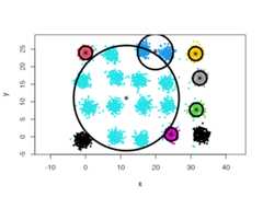
However, using spherical densities (type = 'spherical') on the same data setwill lead to sub-optimal results:

cec<- cec(twenty.gaussians,type="spherical",card.min="1%")plot(cec,asp=1)

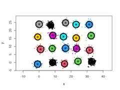
We can help the algorithm identify a more satisfying solution by playing withthesplit.depth andsplit.tries parameters, for instance.

cec<- cec(twenty.gaussians,type="spherical",card.min="1%",split.depth=25,split.tries=15)plot(cec,asp=1)