- Notifications
You must be signed in to change notification settings - Fork162
rougier/numpy-tutorial
Folders and files
| Name | Name | Last commit message | Last commit date | |
|---|---|---|---|---|
Repository files navigation

Sources are available fromgithub.
All code and material is licensed under aCreative CommonsAttribution-ShareAlike 4.0.
NumPy is the fundamental package for scientific computing with Python. Itcontains among other things:
- → a powerful N-dimensional array object
- → sophisticated (broadcasting) functions
- → tools for integrating C/C++ and Fortran code
- → useful linear algebra, Fourier transform, and random number capabilities
Besides its obvious scientific uses, NumPy can also be used as an efficientmulti-dimensional container of generic data. Arbitrary data-types can bedefined and this allows NumPy to seamlessly and speedily integrate with a widevariety of projects. We are going to explore numpy through a simple example,implementing the Game of Life.
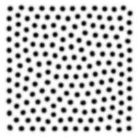
Numpy is slanted toward scientific computing and we'll consider in this sectionthegame of life byJohn Conway which is one of the earliest example of cellular automata (seefigure below). Those cellular automaton can be conveniently considered as arrayof cells that are connected together through the notion of neighbours. We'llshow in the following sections implementation of this game using pure pythonand numpy in order to illustrate main differences with python and numpy.

Figure 1 Simulation of the game of life.
Note
This is an excerpt fromwikipedia entry on CellularAutomaton.
The Game of Life, also known simply as Life, is a cellular automaton devisedby the British mathematician John Horton Conway in 1970. It is thebest-known example of a cellular automaton. The "game" is actually azero-player game, meaning that its evolution is determined by its initialstate, needing no input from human players. One interacts with the Game ofLife by creating an initial configuration and observing how it evolves.
The universe of the Game of Life is an infinite two-dimensional orthogonal gridof square cells, each of which is in one of two possible states, live ordead. Every cell interacts with its eight neighbours, which are the cells thatare directly horizontally, vertically, or diagonally adjacent. At each step intime, the following transitions occur:
- Any live cell with fewer than two live neighbours dies, as if by needs causedby underpopulation.
- Any live cell with more than three live neighbours dies, as if byovercrowding.
- Any live cell with two or three live neighbours lives, unchanged, to the nextgeneration.
- Any dead cell with exactly three live neighbours becomes a live cell.
The initial pattern constitutes the 'seed' of the system. The first generationis created by applying the above rules simultaneously to every cell in the seed– births and deaths happen simultaneously, and the discrete moment at whichthis happens is sometimes called a tick. (In other words, each generation is apure function of the one before.) The rules continue to be applied repeatedlyto create further generations.
We'll first use a very simple setup and more precisely, we'll use theglider pattern that is known tomove one step diagonally in 4 iterations as illustrated below:
 t = 0 |  t = 1 |  t = 2 |  t = 3 |  t = 4 |
This property will help us debug our scripts.
Note
We could have used the more efficientpython array interface but people may be morefamiliar with the list object.
In pure python, we can code the Game of Life using a list of lists representingthe board where cells are supposed to evolve:
>>> Z = [[0,0,0,0,0,0], [0,0,0,1,0,0], [0,1,0,1,0,0], [0,0,1,1,0,0], [0,0,0,0,0,0], [0,0,0,0,0,0]]
This board possesses a0 border that allows to accelerate things a bit byavoiding to have specific tests for borders when counting the number ofneighbours. First step is to count neighbours:
def compute_neigbours(Z): shape = len(Z), len(Z[0]) N = [[0,]*(shape[0]) for i in range(shape[1])] for x in range(1,shape[0]-1): for y in range(1,shape[1]-1): N[x][y] = Z[x-1][y-1]+Z[x][y-1]+Z[x+1][y-1] \ + Z[x-1][y] +Z[x+1][y] \ + Z[x-1][y+1]+Z[x][y+1]+Z[x+1][y+1] return N
To iterate one step in time, we then simply count the number of neighbours foreach internal cell and we update the whole board according to the 4 rules:
def iterate(Z): N = compute_neighbours(Z) for x in range(1,shape[0]-1): for y in range(1,shape[1]-1): if Z[x][y] == 1 and (N[x][y] < 2 or N[x][y] > 3): Z[x][y] = 0 elif Z[x][y] == 0 and N[x][y] == 3: Z[x][y] = 1 return Z
Note
Theshow command is supplied witht he script.
Using a dedicated display function, we can check the program's correct:
>>> show(Z)[0, 0, 1, 0][1, 0, 1, 0][0, 1, 1, 0][0, 0, 0, 0]>>> for i in range(4): iterate(Z)>>> show(Z)[0, 0, 0, 0][0, 0, 0, 1][0, 1, 0, 1][0, 0, 1, 1]
You can download the full script here:game-of-life-python.py
Note
There existsmany more different waysto create a numpy array.
The first thing to do is to create the proper numpy array to hold thecells. This can be done very easily with:
>>> import numpy as np>>> Z = np.array([[0,0,0,0,0,0], [0,0,0,1,0,0], [0,1,0,1,0,0], [0,0,1,1,0,0], [0,0,0,0,0,0], [0,0,0,0,0,0]])
Note
For a complete review on numpy data types, check thedocumentation.
Note that we did not specify thedata type of the array and thus, numpy willchoose one for us. Since all elements are integers, numpy will then choose aninteger data type. This can be easily checked using:
>>> print(Z.dtype)int64
We can also check the shape of the array to make sure it is 6x6:
>>> print(Z.shape)(6, 6)
Each element ofZ can be accessed using arow and acolumnindex (in that order):
>>> print(Z[0,5])0
Note
This element access is actually calledindexing and thisis very powerful tool for vectorized computation.
But even better, we can also access a subpart of the array using the slicenotation:
>>> print(Z[1:5,1:5])[[0 0 1 0] [1 0 1 0] [0 1 1 0] [0 0 0 0]]
In the example above, we actually extract a subpart ofZ ranging from rows 1 to5 and columns 1 to 5. It is important to understand at this point that this isreally a subpart ofZ in the sense that any change to this subpart willhave immediate impact onZ:
>>> A= Z[1:5,1:5]>>> A[0,0]=9>>>print(A)[[9 0 1 0] [1 0 1 0] [0 1 1 0] [0 0 0 0]]>>>print(Z)[[0 0 0 0 0 0] [0 9 0 1 0 0] [0 1 0 1 0 0] [0 0 1 1 0 0] [0 0 0 0 0 0] [0 0 0 0 0 0]]
We set the value ofA[0,0] to 9 and we see immediate change inZ[1,1]becauseA[0,0] actually corresponds toZ[1,1]. This may seem trivialwith such simple arrays, but things can become much more complex (we'll seethat later). If in doubt, you can check easily if an array is part of anotherone:
>>> print(Z.base is None)True>>> print(A.base is Z)True
Note
It is not always possible to vectorize computations and it requiresgenerally some experience. You'll acquire this experience by using numpy (ofcourse) but also by asking questions on themailing list
We now need a function to count the neighbours. We could do it the same way asfor the python version, but this would make things very slow because of thenested loops. We would prefer to act on the whole array whenever possible, thisis calledvectorization.
Ok, let's start then...
First, you need to know that you can manipulateZas if (and onlyasif) it was a regular scalar:
>>> print(1+(2*Z+3))[[4 4 4 4 4 4] [4 4 4 6 4 4] [4 6 4 6 4 4] [4 4 6 6 4 4] [4 4 4 4 4 4] [4 4 4 4 4 4]]
If you look carefully at the output, you may realize that the ouptutcorresponds to the formula above applied individually to each element. Saiddifferently, we have(1+(2*Z+3))[i,j] == (1+(2*Z[i,j]+3)) for any i,j.
Ok, so far, so good. Now what happens if we add Z with one of its subpart,let's sayZ[1:-1,1:-1] ?
>>> Z+ Z[1:-1,1:-1]Traceback (most recent call last):File "<stdin>", line 1, in <module>ValueError: operands could not be broadcast together with shapes (6,6) (4,4)
This raises aValue Error, but more interestingly, numpy complains aboutthe impossibility ofbroadcasting the two arrays together.Broadcasting isa very powerful feature of numpy and most of the time, it saves you a lot ofhassle. Let's consider for example the following code:
>>> print(Z+1)[[1 1 1 1 1 1] [1 1 1 2 1 1] [1 2 1 2 1 1] [1 1 2 2 1 1] [1 1 1 1 1 1] [1 1 1 1 1 1]]
Note
See alsothe broadcasting section in thenumpy documentation.
How can a matrix and a scalar be added together ? Well, they can't. But numpyis smart enough to guess that you actually want to add 1 to each of the elementofZ. This concept of broadcasting is quite powerful and it will take yousome time before masterizing it fully (if even possible).
However, in the present case (counting neighbours if you remember), we won'tuse broadcasting (uh ?). But we'll use vectorize computation using thefollowing code:
>>> N = np.zeros(Z.shape, dtype=int)>>> N[1:-1,1:-1] += (Z[ :-2, :-2] + Z[ :-2,1:-1] + Z[ :-2,2:] + Z[1:-1, :-2] + Z[1:-1,2:] + Z[2: , :-2] + Z[2: ,1:-1] + Z[2: ,2:])
To understand this code, have a look at the figure below:
 |  |  |
 |  |  |
 |  |  |
What we actually did with the above code is to add all the darker blue squarestogether. Since they have been chosen carefully, the result will be exactlywhat we expected. If you want to convince yourself, consider a cell in thelighter blue area of the central sub-figure and check what will the result fora given cell.
Note
Note the use of theravel function that flatten an array. This is necessary since the argwhere function returns flattened indices.
In a first approach, we can write the iterate function using theargwheremethod that will give us the indices where a given condition is True.
def iterate(Z): # Iterate the game of life : naive version # Count neighbours N = np.zeros(Z.shape, int) N[1:-1,1:-1] += (Z[0:-2,0:-2] + Z[0:-2,1:-1] + Z[0:-2,2:] + Z[1:-1,0:-2] + Z[1:-1,2:] + Z[2: ,0:-2] + Z[2: ,1:-1] + Z[2: ,2:]) N_ = N.ravel() Z_ = Z.ravel() # Apply rules R1 = np.argwhere( (Z_==1) & (N_ < 2) ) R2 = np.argwhere( (Z_==1) & (N_ > 3) ) R3 = np.argwhere( (Z_==1) & ((N_==2) | (N_==3)) ) R4 = np.argwhere( (Z_==0) & (N_==3) ) # Set new values Z_[R1] = 0 Z_[R2] = 0 Z_[R3] = Z_[R3] Z_[R4] = 1 # Make sure borders stay null Z[0,:] = Z[-1,:] = Z[:,0] = Z[:,-1] = 0
Even if this first version does not use nested loops, it is far from optimalbecause of the use of the 4 argwhere calls that may be quite slow. We caninstead take advantages of numpy features the following way.
def iterate_2(Z): # Count neighbours N = (Z[0:-2,0:-2] + Z[0:-2,1:-1] + Z[0:-2,2:] + Z[1:-1,0:-2] + Z[1:-1,2:] + Z[2: ,0:-2] + Z[2: ,1:-1] + Z[2: ,2:]) # Apply rules birth = (N==3) & (Z[1:-1,1:-1]==0) survive = ((N==2) | (N==3)) & (Z[1:-1,1:-1]==1) Z[...] = 0 Z[1:-1,1:-1][birth | survive] = 1 return Z
If you look at thebirth andsurvive lines, you'll see that these twovariables are indeed arrays. The right-hand side of these two expressions arein fact logical expressions that will result in boolean arrays (just print themto check). We then set allZ values to 0 (all cells become dead) and we usethebirth andsurvive arrays to conditionally setZ valuesto 1. And we're done ! Let's test this:
>>> print(Z)[[0 0 0 0 0 0] [0 0 0 1 0 0] [0 1 0 1 0 0] [0 0 1 1 0 0] [0 0 0 0 0 0] [0 0 0 0 0 0]]>>> for i in range(4): iterate_2(Z)>>> print(Z)[[0 0 0 0 0 0] [0 0 0 0 0 0] [0 0 0 0 1 0] [0 0 1 0 1 0] [0 0 0 1 1 0] [0 0 0 0 0 0]]
You can download the full script here:game-of-life-numpy.py
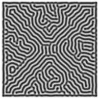
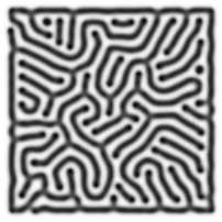
While numpy works perfectly with very small arrays, you'll really benefit fromnumpy power with big to very big arrays. So let us reconsider the game of lifewith a bigger array. First, we won't initalize the array by hand but initalizeit randomly:
>>> Z = np.random.randint(0,2,(256,512))
and we simply iterate as previously:
>>> for i in range(100): iterate(Z)
and display result:
>>> size = np.array(Z.shape)>>> dpi = 72.0>>> figsize= size[1]/float(dpi),size[0]/float(dpi)>>> fig = plt.figure(figsize=figsize, dpi=dpi, facecolor="white")>>> fig.add_axes([0.0, 0.0, 1.0, 1.0], frameon=False)>>> plt.imshow(Z,interpolation='nearest', cmap=plt.cm.gray_r)>>> plt.xticks([]), plt.yticks([])>>> plt.show()

Easy enough, no ?
We have reviewed the very basics of numpy so let's move on to more complex (andmore fun) things.
Note
Description taken from theGray-Scott homepage
Reaction and diffusion of chemical species can produce a variety of patterns,reminiscent of those often seen in nature. The Gray Scott equations model sucha reaction. For more information on this chemical system see the articleComplex Patterns in a Simple System, John E. Pearson, Science, Volume 261,9 July 1993.
Let's consider two chemical speciesU andV with respectiveconcentrationsu andv and diffusion ratesr_u andr_v.V is converted intoP with a rate of conversionk.f represents the rate of the process that feedsUand drainsU,V andP. We can now write:
| Chemical reaction | Equations |
|---|---|
|
|
Obviously, you may think we need two arrays, one forU and forV. ButsinceU andV are tighly linked, it may be indeed better to use asingle array. Numpy allows to do that with the notion ofstructured array:
>>> n = 200>>> Z = np.zeros((n+2,n+2), [('U', np.double), ('V', np.double)])>>> print(Z.dtype)[('U', '<f8'), ('V', '<f8')]The size of the array is (n+2,n+2) since we need the borders when computing theneighbours. However, we'll compute differential equation only in the centerpart, so we can already creates some useful views of this array:
>>> U,V = Z['U'], Z['V']>>> u,v = U[1:-1,1:-1], V[1:-1,1:-1]
Next, we need to compute the Laplacian and we'll use a discrete approximationobtained via thefinite difference method using the same vectorization as for the Game of Life:
def laplacian(Z): return ( Z[0:-2,1:-1] + Z[1:-1,0:-2] - 4*Z[1:-1,1:-1] + Z[1:-1,2:] + Z[2: ,1:-1] )
Finally, we can iterate the computation after choosing some interesting parameters:
for i in range(25000): Lu = laplacian(U) Lv = laplacian(V) uvv = u*v*v u += (Du*Lu - uvv + F *(1-u)) v += (Dv*Lv + uvv - (F+k)*v )
And we're done !
You can download the full script here:gray-scott.py
Here are some exercises, try to do them without looking at the solution (justhighligh the blank part to see it).
Import the numpy package under the name
npimportnumpyasnp
Print the numpy version and the configuration.
print(np.__version__)np.__config__.show()
Hint
Seenp.zeros
Create a null vector of size 10
Z=np.zeros(10)
Create a null vector of size 10 but the fifth value which is 1
Z=np.zeros(10)Z[4]=1
Hint
Seenp.arange
Create a vector with values ranging from 10 to 99
Z=10+np.arange(90)
Create a 3x3 matrix with values ranging from 0 to 8
Z=np.arange(9).reshape(3,3)
Hint
Seenp.nonzero
Find indices of non-zero elements from [1,2,0,0,4,0]
print(np.nonzero([1,2,0,0,4,0]))
Declare a 3x3 identity matrix
Z=np.eye(3)
Declare a 5x5 matrix with values 1,2,3,4 just below the diagonal
Z=np.diag(1+np.arange(4),k=-1)
Hint
Declare a 10x10x10 array with random values
Z=np.random.random((10,10,10))
Declare a 8x8 matrix and fill it with a checkerboard pattern
Z=np.zeros((8,8))Z[1::2,::2]=1Z[::2,1::2]=1
Declare a 10x10 array with random values and find the minimum and maximum values
Z=np.random.random((10,10,10))Zmin,Zmax=Z.min(),Z.max()
Create a checkerboard 8x8 matrix using the tile function
Z=np.tile(np.array([[0,1],[1,0]]), (4,4))
Normalize a 5x5 random matrix (between 0 and 1)
Z=np.random.random((5,5))Zmax,Zmin=Z.max(),Z.min()Z= (Z-Zmin)/(Zmax-Zmin)
Hint
See thelinear algebra documentation
Multiply a 5x3 matrix by a 3x2 matrix (real matrix product)
Z=np.dot(np.ones((5,3)),np.ones((3,2)))
Create a 10x10 matrix with row values ranging from 0 to 9
Z=np.zeros((10,10))Z+=np.arange(10)
Create a vector of size 1000 with values ranging from 0 to 1, both excluded
Z=np.random.linspace(0,1,1002,endpoint=True)[1:-1]
Create a random vector of size 100 and sort it
Z=np.random.random(100)Z.sort()
Consider two random matrices A anb B, check if they are equal.
A=np.random.randint(0,2,(2,2))B=np.random.randint(0,2,(2,2))equal=np.allclose(A,B)
Create a random vector of size 1000 and find the mean value
Z=np.random.random(1000)m=Z.mean()
Consider a random 100x2 matrix representing cartesian coordinates, convertthem to polar coordinates
Z=np.random.random((100,2))X,Y=Z[:,0],Z[:,1]R=np.sqrt(X**2+Y**2)T=np.arctan2(Y,X)
Create random vector of size 100 and replace the maximum value by 0
Z=np.random.random(100)Z[Z.argmax()]=0
Hint
See the documentation onStructured arrays
Declare a structured array with
xandycoordinates covering the[0,1]x[0,1] area.Z=np.zeros((10,10), [('x',float),('y',float)])Z['x'],Z['y']=np.meshgrid(np.linspace(0,1,10),np.linspace(0,1,10))
Hint
Have a look atData type routines
Print the minimum and maximum representable value for each numpy scalar type
fordtypein [np.int8,np.int32,np.int64]:print(np.iinfo(dtype).min)print(np.iinfo(dtype).max)fordtypein [np.float32,np.float64]:print(np.finfo(dtype).min)print(np.finfo(dtype).max)print(np.finfo(dtype).eps)
Create a structured array representing a position (x,y) and a color (r,g,b)
Z=np.zeros(10, [ ('position', [ ('x',float,1), ('y',float,1)]), ('color', [ ('r',float,1), ('g',float,1), ('b',float,1)])])
Consider a random vector with shape (100,2) representing coordinates, findpoint by point distances
Z=np.random.random((10,2))X,Y=np.atleast_2d(Z[:,0]),np.atleast_2d(Z[:,1])D=np.sqrt( (X-X.T)**2+ (Y-Y.T)**2)
Generate a generic 2D Gaussian-like array
X,Y=np.meshgrid(np.linspace(-1,1,100),np.linspace(-1,1,100))D=np.sqrt(X*X+Y*Y)sigma,mu=1.0,0.0G=np.exp(-( (D-mu)**2/ (2.0*sigma**2 ) ) )
Consider the vector [1, 2, 3, 4, 5], how to build a new vector with 3consecutive zeros interleaved between each value ?
Z=np.array([1,2,3,4,5])nz=3Z0=np.zeros(len(Z)+ (len(Z)-1)*(nz))Z0[::nz+1]=Z
Numpy benefits from extensive documentation as well as a large community ofusers and developpers. Here are some links of interest:
The SciPy Lecture notes offers a teaching material on the scientific Pythonecosystem as well as quick introduction to central tools and techniques. Thedifferent chapters each correspond to a 1 to 2 hours course with increasinglevel of expertise, from beginner to expert.
- Prerequisites
- The Basics
- Shape Manipulation
- Copies and Views
- Less Basic
- Fancy indexing and index tricks
- Linear Algebra
- Tricks and Tips
A first-aid kit for the numerically adventurous by Stéfan van der Walt.
An introduction to Numpy and Scipy
A short introduction to Numpy and Scipy by M. Scott Shell.
This guide is intended as an introductory overview of NumPy and explains howto install and make use of the most important features of NumPy.
This reference manual details functions, modules, and objects included inNumpy, describing what they are and what they do.
- General questions about numpy
- General questions about SciPy
- Basic SciPy/numpy usage
- Advanced NumPy/SciPy usage
- NumPy/SciPy installation
- Miscellaneous Issues
The code is fairly well documented and you can quickly access a specificcommand from within a python session:
>>> import numpy as np>>> help(np.ones)Help on function ones in module numpy.core.numeric:ones(shape, dtype=None, order='C') Return a new array of given shape and type, filled with ones. Please refer to the documentation for `zeros` for further details. See Also -------- zeros, ones_like Examples -------- >>> np.ones(5) array([ 1., 1., 1., 1., 1.]) >>> np.ones((5,), dtype=np.int) array([1, 1, 1, 1, 1]) >>> np.ones((2, 1)) array([[ 1.], [ 1.]]) >>> s = (2,2) >>> np.ones(s) array([[ 1., 1.], [ 1., 1.]])
Finally, there is amailing list where you canask for help.
| Data type | Description |
|---|---|
| bool | Boolean (True or False) stored as a byte |
| int | Platform integer (normally either int32 or int64) |
| int8 | Byte (-128 to 127) |
| int16 | Integer (-32768 to 32767) |
| int32 | Integer (-2147483648 to 2147483647) |
| int64 | Integer (9223372036854775808 to 9223372036854775807) |
| uint8 | Unsigned integer (0 to 255) |
| uint16 | Unsigned integer (0 to 65535) |
| uint32 | Unsigned integer (0 to 4294967295) |
| uint64 | Unsigned integer (0 to 18446744073709551615) |
| float | Shorthand for float64. |
| float16 | Half precision float: sign bit, 5 bits exponent, 10 bits mantissa |
| float32 | Single precision float: sign bit, 8 bits exponent, 23 bits mantissa |
| float64 | Double precision float: sign bit, 11 bits exponent, 52 bits mantissa |
| complex | Shorthand for complex128. |
| complex64 | Complex number, represented by two 32-bit floats |
| complex128 | Complex number, represented by two 64-bit floats |
| Code | Result | Code | Result | |
|---|---|---|---|---|
Z = zeros(9) |  | Z = zeros((5,9)) |  | |
Z = ones(9) |  | Z = ones((5,9)) |  | |
Z = array( [0,0,0,0,0,0,0,0,0] ) |  | Z = array( [[0,0,0,0,0,0,0,0,0], [0,0,0,0,0,0,0,0,0], [0,0,0,0,0,0,0,0,0], [0,0,0,0,0,0,0,0,0], [0,0,0,0,0,0,0,0,0]]) |  | |
Z = arange(9) |  | Z = arange(5*9).reshape(5,9) |  | |
Z = random.uniform(0,1,9) |  | Z = random.uniform(0,1,(5,9)) |  |
| Code | Result | Code | Result |
|---|---|---|---|
Z[2,2] = 1 |  | Z = Z.reshape(1,12) | .png) |
Z = Z.reshape(4,3) | .png) | Z = Z.reshape(12,1) | .png) |
Z = Z.reshape(6,2) | .png) | ||
Z = Z.reshape(2,6) | .png) |
| Code | Result | Code | Result | |
|---|---|---|---|---|
Z |  | Z[...] = 1 | ![figures/slice-Z[...].png](/mt/?noimg=&dark=on&url=https%3a%2f%2fgithub.com%2frougier%2fnumpy-tutorial%2fblob%2fmaster%2ffigures%2fslice-Z%5b...%5d.png) | |
Z[1,1] = 1 | ![figures/slice-Z[1,1].png](/mt/?noimg=&dark=on&url=https%3a%2f%2fgithub.com%2frougier%2fnumpy-tutorial%2fblob%2fmaster%2ffigures%2fslice-Z%5b1%2c1%5d.png) | Z[:,0] = 1 | ![figures/slice-Z[:,0].png](/mt/?noimg=&dark=on&url=https%3a%2f%2fgithub.com%2frougier%2fnumpy-tutorial%2fblob%2fmaster%2ffigures%2fslice-Z%5b%3a%2c0%5d.png) | |
Z[0,:] = 1 | ![figures/slice-Z[0,:].png](/mt/?noimg=&dark=on&url=https%3a%2f%2fgithub.com%2frougier%2fnumpy-tutorial%2fblob%2fmaster%2ffigures%2fslice-Z%5b0%2c%3a%5d.png) | Z[2:,2:] = 1 | ![figures/slice-Z[2:,2:].png](/mt/?noimg=&dark=on&url=https%3a%2f%2fgithub.com%2frougier%2fnumpy-tutorial%2fblob%2fmaster%2ffigures%2fslice-Z%5b2%3a%2c2%3a%5d.png) | |
Z[:,::2] = 1 | ![figures/slice-Z[:,::2].png](/mt/?noimg=&dark=on&url=https%3a%2f%2fgithub.com%2frougier%2fnumpy-tutorial%2fblob%2fmaster%2ffigures%2fslice-Z%5b%3a%2c%3a%3a2%5d.png) | Z[::2,:] = 1 | ![figures/slice-Z[::2,:].png](/mt/?noimg=&dark=on&url=https%3a%2f%2fgithub.com%2frougier%2fnumpy-tutorial%2fblob%2fmaster%2ffigures%2fslice-Z%5b%3a%3a2%2c%3a%5d.png) | |
Z[:-2,:-2] = 1 | ![figures/slice-Z[:-2,:-2].png](/mt/?noimg=&dark=on&url=https%3a%2f%2fgithub.com%2frougier%2fnumpy-tutorial%2fblob%2fmaster%2ffigures%2fslice-Z%5b%3a-2%2c%3a-2%5d.png) | Z[2:4,2:4] = 1 | ![figures/slice-Z[2:4,2:4].png](/mt/?noimg=&dark=on&url=https%3a%2f%2fgithub.com%2frougier%2fnumpy-tutorial%2fblob%2fmaster%2ffigures%2fslice-Z%5b2%3a4%2c2%3a4%5d.png) | |
Z[::2,::2] = 1 | ![figures/slice-Z[::2,::2].png](/mt/?noimg=&dark=on&url=https%3a%2f%2fgithub.com%2frougier%2fnumpy-tutorial%2fblob%2fmaster%2ffigures%2fslice-Z%5b%3a%3a2%2c%3a%3a2%5d.png) | Z[3::2,3::2] = 1 | ![figures/slice-Z[3::2,3::2].png](/mt/?noimg=&dark=on&url=https%3a%2f%2fgithub.com%2frougier%2fnumpy-tutorial%2fblob%2fmaster%2ffigures%2fslice-Z%5b3%3a%3a2%2c3%3a%3a2%5d.png) |
 | + |  | → | | + |  | = |  |
 | + |  | → | | + |  | = |  |
 | + |  | → | | + |  | = |  |
 | + |  | → |  | + |  | = |  |
| Code | Before | After |
|---|---|---|
Z = np.where(Z > 0.5, 0, 1) |  |  |
Z = np.maximum(Z, 0.5) |  |  |
Z = np.minimum(Z, 0.5) |  |  |
Z = np.sum(Z, axis=0) |  |  |
About
Numpy beginner tutorial
Topics
Resources
Uh oh!
There was an error while loading.Please reload this page.
Stars
Watchers
Forks
Packages0
Uh oh!
There was an error while loading.Please reload this page.