- Notifications
You must be signed in to change notification settings - Fork183
Text mining using tidy tools ✨📄✨
License
juliasilge/tidytext
Folders and files
| Name | Name | Last commit message | Last commit date | |
|---|---|---|---|---|
Repository files navigation
Authors:Julia Silge,DavidRobinson
License:MIT
Usingtidy data principles canmake many text mining tasks easier, more effective, and consistent withtools already in wide use. Much of the infrastructure needed for textmining with tidy data frames already exists in packages likedplyr,broom,tidyr, andggplot2. In this package,we provide functions and supporting data sets to allow conversion oftext to and from tidy formats, and to switch seamlessly between tidytools and existing text mining packages. Check outourbook to learn more about text miningusing tidy data principles.
You can install this package from CRAN:
install.packages("tidytext")Or you can install the development version from GitHub withremotes:
library(remotes)install_github("juliasilge/tidytext")
The novels of Jane Austen can be so tidy! Let’s use the text of JaneAusten’s 6 completed, published novels from thejaneaustenr package,and transform them to a tidy format. janeaustenr provides them as aone-row-per-line format:
library(janeaustenr)library(dplyr)original_books<- austen_books()|> group_by(book)|> mutate(line= row_number())|> ungroup()original_books#> # A tibble: 73,422 × 3#> text book line#> <chr> <fct> <int>#> 1 "SENSE AND SENSIBILITY" Sense & Sensibility 1#> 2 "" Sense & Sensibility 2#> 3 "by Jane Austen" Sense & Sensibility 3#> 4 "" Sense & Sensibility 4#> 5 "(1811)" Sense & Sensibility 5#> 6 "" Sense & Sensibility 6#> 7 "" Sense & Sensibility 7#> 8 "" Sense & Sensibility 8#> 9 "" Sense & Sensibility 9#> 10 "CHAPTER 1" Sense & Sensibility 10#> # ℹ 73,412 more rows
To work with this as a tidy dataset, we need to restructure it asone-token-per-row format. Theunnest_tokens() function is a way toconvert a dataframe with a text column to be one-token-per-row:
library(tidytext)tidy_books<-original_books|> unnest_tokens(word,text)tidy_books#> # A tibble: 725,055 × 3#> book line word#> <fct> <int> <chr>#> 1 Sense & Sensibility 1 sense#> 2 Sense & Sensibility 1 and#> 3 Sense & Sensibility 1 sensibility#> 4 Sense & Sensibility 3 by#> 5 Sense & Sensibility 3 jane#> 6 Sense & Sensibility 3 austen#> 7 Sense & Sensibility 5 1811#> 8 Sense & Sensibility 10 chapter#> 9 Sense & Sensibility 10 1#> 10 Sense & Sensibility 13 the#> # ℹ 725,045 more rows
This function uses thetokenizers package to separateeach line into words. The default tokenizing is for words, but otheroptions include characters, n-grams, sentences, lines, paragraphs, orseparation around a regex pattern.
Now that the data is in a one-word-per-row format, we can manipulate itwith tidy tools like dplyr. We can remove stop words (available via thefunctionget_stopwords()) with ananti_join().
tidy_books<-tidy_books|> anti_join(get_stopwords())
We can also usecount() to find the most common words in all the booksas a whole.
tidy_books|> count(word,sort=TRUE)#> # A tibble: 14,375 × 2#> word n#> <chr> <int>#> 1 mr 3015#> 2 mrs 2446#> 3 must 2071#> 4 said 2041#> 5 much 1935#> 6 miss 1855#> 7 one 1831#> 8 well 1523#> 9 every 1456#> 10 think 1440#> # ℹ 14,365 more rows
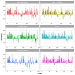
Sentiment analysis can be implemented as an inner join. Three sentimentlexicons are available via theget_sentiments() function. Let’sexamine how sentiment changes across each novel. Let’s find a sentimentscore for each word using the Bing lexicon, then count the number ofpositive and negative words in defined sections of each novel.
library(tidyr)get_sentiments("bing")#> # A tibble: 6,786 × 2#> word sentiment#> <chr> <chr>#> 1 2-faces negative#> 2 abnormal negative#> 3 abolish negative#> 4 abominable negative#> 5 abominably negative#> 6 abominate negative#> 7 abomination negative#> 8 abort negative#> 9 aborted negative#> 10 aborts negative#> # ℹ 6,776 more rowsjaneaustensentiment<-tidy_books|> inner_join( get_sentiments("bing"),by="word",relationship="many-to-many" )|> count(book,index=line%/%80,sentiment)|> pivot_wider(names_from=sentiment,values_from=n,values_fill=0)|> mutate(sentiment=positive-negative)janeaustensentiment#> # A tibble: 920 × 5#> book index negative positive sentiment#> <fct> <dbl> <int> <int> <int>#> 1 Sense & Sensibility 0 16 32 16#> 2 Sense & Sensibility 1 19 53 34#> 3 Sense & Sensibility 2 12 31 19#> 4 Sense & Sensibility 3 15 31 16#> 5 Sense & Sensibility 4 16 34 18#> 6 Sense & Sensibility 5 16 51 35#> 7 Sense & Sensibility 6 24 40 16#> 8 Sense & Sensibility 7 23 51 28#> 9 Sense & Sensibility 8 30 40 10#> 10 Sense & Sensibility 9 15 19 4#> # ℹ 910 more rows
Now we can plot these sentiment scores across the plot trajectory ofeach novel.
library(ggplot2)ggplot(janeaustensentiment, aes(index,sentiment,fill=book))+ geom_col(show.legend=FALSE)+ facet_wrap(vars(book),ncol=2,scales="free_x")
For more examples of text mining using tidy data frames, see thetidytext vignette.
Some existing text mining datasets are in the form of aDocumentTermMatrix class (from the tm package). For example, considerthe corpus of 2246 Associated Press articles from the topicmodelsdataset.
library(tm)data("AssociatedPress",package="topicmodels")AssociatedPress#> <<DocumentTermMatrix (documents: 2246, terms: 10473)>>#> Non-/sparse entries: 302031/23220327#> Sparsity : 99%#> Maximal term length: 18#> Weighting : term frequency (tf)
If we want to analyze this with tidy tools, we need to transform it intoa one-row-per-term data frame first with atidy() function. (For moreon the tidy verb,see the broompackage).
tidy(AssociatedPress)#> # A tibble: 302,031 × 3#> document term count#> <int> <chr> <dbl>#> 1 1 adding 1#> 2 1 adult 2#> 3 1 ago 1#> 4 1 alcohol 1#> 5 1 allegedly 1#> 6 1 allen 1#> 7 1 apparently 2#> 8 1 appeared 1#> 9 1 arrested 1#> 10 1 assault 1#> # ℹ 302,021 more rows
We could find the most negative documents:
ap_sentiments<- tidy(AssociatedPress)|> inner_join(get_sentiments("bing"),by= c(term="word"))|> count(document,sentiment,wt=count)|> pivot_wider(names_from=sentiment,values_from=n,values_fill=0)|> mutate(sentiment=positive-negative)|> arrange(sentiment)
Or we can join the Austen and AP datasets and compare the frequencies ofeach word:
comparison<- tidy(AssociatedPress)|> count(word=term)|> rename(AP=n)|> inner_join(count(tidy_books,word))|> rename(Austen=n)|> mutate(AP=AP/ sum(AP),Austen=Austen/ sum(Austen) )comparison#> # A tibble: 4,730 × 3#> word AP Austen#> <chr> <dbl> <dbl>#> 1 abandoned 0.000170 0.00000493#> 2 abide 0.0000291 0.0000197#> 3 abilities 0.0000291 0.000143#> 4 ability 0.000238 0.0000148#> 5 able 0.000664 0.00151#> 6 abroad 0.000194 0.000178#> 7 abrupt 0.0000291 0.0000247#> 8 absence 0.0000776 0.000547#> 9 absent 0.0000436 0.000247#> 10 absolute 0.0000533 0.000128#> # ℹ 4,720 more rowslibrary(scales)ggplot(comparison, aes(AP,Austen))+ geom_point(alpha=0.5)+ geom_text(aes(label=word),check_overlap=TRUE,vjust=1,hjust=1)+ scale_x_log10(labels= percent_format())+ scale_y_log10(labels= percent_format())+ geom_abline(color="red")
<img src=“man/figures/README-unnamed-chunk-13-1.png” alt=“Scatterplotfor word frequencies in Jane Austen vs. AP news articles. Some wordslike”cried” are only common in Jane Austen, some words like “national”are only common in AP articles, and some word like “time” are common inboth.” width=“100%” />
For more examples of working with objects from other text miningpackages using tidy data principles, see thevignetteon converting to and from document term matrices.
This project is released with aContributor Code ofConduct.By participating in this project you agree to abide by its terms.Feedback, bug reports (and fixes!), and feature requests are welcome;file issues or seek supporthere.
About
Text mining using tidy tools ✨📄✨
Topics
Resources
License
Uh oh!
There was an error while loading.Please reload this page.
Stars
Watchers
Forks
Packages0
Uh oh!
There was an error while loading.Please reload this page.

