- Notifications
You must be signed in to change notification settings - Fork0
Calculate Earth’s Obliquity and Precession in the Past
License
japhir/snvecR
Folders and files
| Name | Name | Last commit message | Last commit date | |
|---|---|---|---|---|
Repository files navigation
Easily calculate precession and obliquity from an astronomical solution(AS, defaults to ZB18a from Zeebe and Lourens (2019)) and assumed orreconstructed values for dynamical ellipticity (Ed) and tidaldissipation (Td). This is a translation and adaptation of theC-code in the supplementary material to Zeebe and Lourens (2022), withfurther details on the methodology described in Zeebe (2022). The nameof the C-routine is snvec, which refers to the key units of computation:spin vector s and orbit normal vector n.
You can install snvecR like so:
install.packages("snvecR")To use the development version of the package, use:
remotes::install_github("japhir/snvecR")
Then load it with:
library(snvecR)The functionget_solution() easily downloads astronomical solutionsfromRichard Zeebe’swebsiteand stores them locally so that they can be reused conveniently. Notethat when run interactively, the function will ask for confirmation tostore the files to the cache directory (which can be customized withoptions(snvecR.cachedir = "/path/to/cache")). See the documentationfor more information (?snvecR::get_solution).
# full solution needed for snvec belowsol<- get_solution("full-ZB18a")#> ℹ The astronomical solution "full-ZB18a" has not been cached.#> ℹ Reading 'full-ZB18a.dat' from website <http://www.soest.hawaii.edu/oceanography/faculty/zeebe_files/Astro/PrecTilt/OS/ZB18a/ems-plan3.dat>.#> ℹ Calculating helper columns.#> ℹ The cache directory is '/tmp/Rtmp6SR5fp/snvecR9d10d4db377ba'.#> ℹ Saved astronomical solution with helper columns 'full-ZB18a.rds' to cache.#> ℹ Future calls to `get_solution("full-ZB18a")` will read from the cache.#> ! If you want to read from scratch, specify `force = TRUE`.# eccentricity solutionsZB18a<- get_solution("ZB18a-300")#> ℹ The astronomical solution "ZB18a-300" has not been cached.#> ℹ Reading 'ZB18a-300.dat' from website <http://www.soest.hawaii.edu/oceanography/faculty/zeebe_files/Astro/300Myr/ZB18a.dat>.#> ℹ Flipped time for "ZB18a-300" so that it is in negative kyr.#> ℹ The cache directory is '/tmp/Rtmp6SR5fp/snvecR9d10d4db377ba'.#> ℹ Saved astronomical solution with helper columns 'ZB18a-300.rds' to cache.#> ℹ Future calls to `get_solution("ZB18a-300")` will read from the cache.#> ! If you want to read from scratch, specify `force = TRUE`.ZB20a<- get_solution("ZB20a")#> ℹ The astronomical solution "ZB20a" has not been cached.#> ℹ Reading 'ZB20a.dat' from website <http://www.soest.hawaii.edu/oceanography/faculty/zeebe_files/Astro/300Myr/ZB20a.dat>.#> ℹ Flipped time for "ZB20a" so that it is in negative kyr.#> ℹ The cache directory is '/tmp/Rtmp6SR5fp/snvecR9d10d4db377ba'.#> ℹ Saved astronomical solution with helper columns 'ZB20a.rds' to cache.#> ℹ Future calls to `get_solution("ZB20a")` will read from the cache.#> ! If you want to read from scratch, specify `force = TRUE`.# a pre-computed precession-tilt solution (PT)ZB18a_1_1<- get_solution("PT-ZB18a(1,1)")#> ℹ The astronomical solution "PT-ZB18a(1.0000,1.0000)" has not been cached.#> ℹ Reading 'PT-ZB18a(1.0000,1.0000).dat' from website <http://www.soest.hawaii.edu/oceanography/faculty/zeebe_files/Astro/PrecTilt/ZB18a/asc/PT.De1.0000Td1.0000.dat>.#> ℹ The cache directory is '/tmp/Rtmp6SR5fp/snvecR9d10d4db377ba'.#> ℹ Saved astronomical solution with helper columns 'PT-ZB18a(1.0000,1.0000).rds'#> to cache.#> ℹ Future calls to `get_solution("PT-ZB18a(1.0000,1.0000)")` will read from the#> cache.#> ! If you want to read from scratch, specify `force = TRUE`.
# the 3.5 Gyr solutions, e.g. number 5ZB23.R05<- get_solution("ZB23.R05")#> ℹ The astronomical solution "ZB23.R05" has not been cached.#> ℹ Reading 'ZB23.R05.dat' from website <http://www.soest.hawaii.edu/oceanography/faculty/zeebe_files/Astro/3.5Gyr/ZB23-N64-eiop/ZB23.R05.eiop.dat.zip>.#> Downloading any of the ZB23.RXX solutions will take some time.#> Zip files are about 154 MB.#> Continue downloading and caching? (Yes/no/cancel)#> ℹ The cache directory is '/home/japhir/.cache/R/snvecR'.#> ℹ Saved astronomical solution with helper columns 'ZB23.R05.rds' to cache.#> ℹ Future calls to `get_solution("ZB23.R05")` will read from the cache.#> ! If you want to read from scratch, specify `force = TRUE`.
Here’s thesnvec() function that calculates climatic precession andobliquity from an orbital solution input and values for tidaldissipation (Td) and dynamical ellipticity (Ed).
solution<- snvec(tend=-1000,# final timestep in kyred=1,# dynamical ellipticity, normalized to moderntd=0,# tidal dissipation, normalized to modernastronomical_solution="full-ZB18a",# see ?full_ZB18a for detailstres=-0.4# timestep resolution in kyr (so this is 400 years) )#> This is snvecR VERSION: 3.10.1.9000 2025-03-10#> Richard E. Zeebe#> Ilja J. Kocken#>#> Integration parameters:#> • `tend` = -1000 kyr#> • `ed` = 1#> • `td` = 0#> • `astronomical_solution` = "full-ZB18a"#> • `os_ref_frame` = "HCI"#> • `os_omt` = defaulting to 75.594#> • `os_inct` = defaulting to 7.155#> • `tres` = -0.4 kyr#> • `atol` = 1e-05#> • `rtol` = 0#> • `solver` = "vode"#> ℹ started at "2025-03-10 13:24:07.819133"#> Final values:#> • s[1][2][3]: 0.404184487124565, -0.0537555129057148, and 0.913036138471423#> • s-error = |s|-1: -5.51290422495798e-05#> Final values:#> • obliquity: 0.413060472710089 rad#> • precession: -0.562357122261026 rad#> ℹ stopped at "2025-03-10 13:24:08.522222"#> ℹ total duration: 0.7
To quickly save out the results for further study to CSV1:
write.csv(solution,"ZB18a_ed-1.0_td-0.0.csv")
see?snvec for further documentation.
Here we create a quick plot of the obliquity:
plot(epl~time,data=solution,type='l')
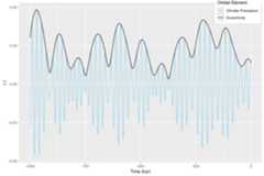
Or if you want to make a slightly fancier plot of the calculatedclimatic precession with the eccentricity envelope:
library(ggplot2)solution|> ggplot(aes(x=time,y=cp))+ labs(x="Time (kyr)",y="(-)",colour="Orbital Element")+# plot climatic precession geom_line(aes(colour="Climatic Precession"))+# add the eccentricity envelope geom_line(aes(y=ee,colour="Eccentricity"),data= get_solution()|>dplyr::filter(time>-1000))+ scale_color_discrete(type= c("skyblue","black"))+ theme(legend.position="inside",legend.position.inside= c(.9,.95))
Contributions are more than welcome! If something doesn’t work the wayyou expect and you don’t know how to fix it,write anissue. If you do know how tofix it, feel free tocreate a pullrequest!
Zeebe, R. E., & Lourens, L. J. (2019). Solar System chaos and thePaleocene–Eocene boundary age constrained by geology and astronomy.Science, 365(6456), 926–929.doi:10.1126/science.aax0612.
Zeebe, R. E., & Lourens, L. J. (2022). A deep-time dating tool forpaleo-applications utilizing obliquity and precession cycles: The roleof dynamical ellipticity and tidal dissipation.Paleoceanography andPaleoclimatology, e2021PA004349.doi:10.1029/2021PA004349.
Zeebe, R. E. (2022). Reduced Variations in Earth’s and Mars’ OrbitalInclination and Earth’s Obliquity from 58 to 48 Myr ago due to SolarSystem Chaos.The Astronomical Journal, 164(3),doi:10.3847/1538-3881/ac80f8.
Wikipedia page on Orbital Elements:https://en.wikipedia.org/wiki/Orbital_elements
Footnotes
Actually I would recommend the
readrpackage withreadr::write_csv()instead.↩
About
Calculate Earth’s Obliquity and Precession in the Past
Resources
License
Uh oh!
There was an error while loading.Please reload this page.
Stars
Watchers
Forks
Packages0
Uh oh!
There was an error while loading.Please reload this page.

