Folders and files

Name		Name	Last commit message	Last commit date
Latest commit History 167 Commits
.github		.github
R		R
data-raw		data-raw
data		data
explore		explore
inst		inst
man		man
src		src
tests		tests
vignettes		vignettes
.Rbuildignore		.Rbuildignore
.gitignore		.gitignore
DESCRIPTION		DESCRIPTION
LICENSE.md		LICENSE.md
NAMESPACE		NAMESPACE
NEWS.md		NEWS.md
README.Rmd		README.Rmd
README.md		README.md
_pkgdown.yml		_pkgdown.yml
birdie.Rproj		birdie.Rproj
cran-comments.md		cran-comments.md

Repository files navigation

BIRDiE: Estimating disparities when race is not observed

Bayesian Improved Surname Geocoding (BISG) is a simple model thatpredicts individual race based off last names and addresses. Whilepredictive, it is not perfect, and measurement error in thesepredictions can cause problems in downstream analyses.

Bayesian Instrumental Regression for Disparity Estimation (BIRDiE) is aclass of Bayesian models for accurately estimating conditionaldistributions by race, using BISG probabilities as inputs. This packageimplements BIRDiE as described inMcCartan, Fisher, Goldin, Ho, andImai (2025). It alsoimplements standard BISG and an improved measurement-error BISG model asdescribed inImai, Olivella, and Rosenman(2022).

Do I need BIRDiE?

BIRDiE is a statistical model to let you estimate the average value of a variable in different racial groups.To take an example from our research paper, if your data are tax records and you want to estimate the rate at which different racial groups take a certain tax credit, BIRDiE can help you do that.

BIRDiE is applied on top of individual-level imputations/predictions of race from methods like BISG.If your only goal is to estimate individual race probabilities, then BIRDiE is not helpful—BISG alone suffices.The graphic below gives an overview of the problem BIRDiE solves and how it fits together with existing methods.

What is the difference between BIRDiE and BISG?

BISG is a simple model that estimates the probability of each individual belonging to diferent racial groups, based on their last name and/or residence location.

BIRDiE is a statistical model that takes race probabilities (like BISG) asinputs to estimate the average value of an outcome variable in different racial groups.If your research question involves both race and another (outcome) variable, then you likely need to apply BIRDiE on top of BISG to avoid biases caused by measurement error in BISG predictions.

Is BIRDiE better than BISG, fBISG, etc?

There are many methods for imputing or predicting individual race, including BISG, fBISG, and others.Mainly, these methods use different data sources or slightly different models.

BIRDiE isnot a replacement for these methods, but rather a complementary tool that uses the outputs of these methods to properly estimate disparities in other variables.When BIRDiE is applied on top of these methods, it generally produces far more accurate estimates than directly thresholding or weighting by the outputs of the prediction methods alone.

Do I have to use thebirdie software to do BISG?

Thebirdie software includes, for convenience, an implementation of basic BISG.More complicated BISG models that use more data are possible usingbirdie, but may be easier with other software packages, such aswru.The BIRDiE method, found in thebirdie() function here, can take race predictions fromany software package as inputs.

Installation

You can install the latest version of the package from CRAN with:

install.packages("birdie")

You can also install the development version with:

# install.packages("remotes")remotes::install_github("CoryMcCartan/birdie")

Basic Usage

A basic analysis has two steps. First, you compute BISG probabilityestimates with thebisg() orbisg_me() functions (or using any otherprobabilistic race prediction tool). Then, you estimate the distributionof an outcome variable by race using thebirdie() function.

library(birdie)data(pseudo_vf)head(pseudo_vf)#> # A tibble: 6 × 4#>   last_name zip   race  turnout#>   <fct>     <fct> <fct> <fct>#> 1 BEAVER    28748 white yes#> 2 WILLIAMS  28144 black no#> 3 ROSEN     28270 white yes#> 4 SMITH     28677 black yes#> 5 FAY       28748 white no#> 6 CHURCH    28215 white yes

To compute BISG probabilities, you provide the last name and(optionally) geography variables as part of a formula.

r_probs= bisg(~ nm(last_name)+ zip(zip),data=pseudo_vf)head(r_probs)#> # A tibble: 6 × 6#>   pr_white pr_black pr_hisp pr_asian  pr_aian pr_other#>      <dbl>    <dbl>   <dbl>    <dbl>    <dbl>    <dbl>#> 1    0.956  0.00371  0.0103 0.000674 0.00886    0.0202#> 2    0.162  0.795    0.0122 0.00102  0.000873   0.0292#> 3    0.943  0.00378  0.0218 0.0107   0.000386   0.0202#> 4    0.569  0.365    0.0302 0.00114  0.00108    0.0339#> 5    0.971  0.00118  0.0131 0.00149  0.00118    0.0125#> 6    0.524  0.315    0.0909 0.00598  0.00255    0.0610

Computing regression estimates requires specifying a model structure.Here, we’ll use a Categorical-Dirichlet regression model that lets therelationship between turnout and race vary by ZIP code. This is the“no-pooling” model from McCartan et al. We’ll use Gibbs sampling forinference, which will also let us capture the uncertainty in ourestimates.

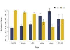
fit= birdie(r_probs,turnout~ proc_zip(zip),data=pseudo_vf,family=cat_dir(),algorithm="gibbs")#> Using weakly informative empirical Bayes prior for Pr(Y | R)#> This message is displayed once every 8 hours.print(fit)#> Categorical-Dirichlet BIRDiE model#> Formula: turnout ~ proc_zip(zip)#>    Data: pseudo_vf#> Number of obs: 5,000#> Estimated distribution:#>     white black  hisp asian  aian other#> no  0.293  0.34 0.372 0.569 0.685 0.499#> yes 0.707  0.66 0.628 0.431 0.315 0.501

Theproc_zip() function fills in missing ZIP codes, among otherthings. We can extract the estimated conditional distributions withcoef(). We can also get updated BISG probabilities that additionallycondition on turnout usingfitted(). Additional functions allow us toextract a tidy version of our estimates (tidy()) and visualize theestimated distributions (plot()).

coef(fit)#>         white     black      hisp     asian      aian     other#> no  0.2934753 0.3403649 0.3720582 0.5687325 0.6847874 0.4994076#> yes 0.7065247 0.6596351 0.6279418 0.4312675 0.3152126 0.5005924head(fitted(fit))#> # A tibble: 6 × 6#>   pr_white pr_black pr_hisp pr_asian  pr_aian pr_other#>      <dbl>    <dbl>   <dbl>    <dbl>    <dbl>    <dbl>#> 1   0.961   0.00349 0.0101  0.000523 0.00577    0.0195#> 2   0.0765  0.893   0.00814 0.00102  0.00106    0.0207#> 3   0.932   0.00542 0.0287  0.00538  0.000384   0.0286#> 4   0.587   0.352   0.0260  0.000833 0.000783   0.0335#> 5   0.945   0.00224 0.0219  0.00368  0.00334    0.0238#> 6   0.528   0.324   0.0895  0.00379  0.00143    0.0538tidy(fit)#> # A tibble: 12 × 3#>    turnout race  estimate#>    <chr>   <chr>    <dbl>#>  1 no      white    0.293#>  2 yes     white    0.707#>  3 no      black    0.340#>  4 yes     black    0.660#>  5 no      hisp     0.372#>  6 yes     hisp     0.628#>  7 no      asian    0.569#>  8 yes     asian    0.431#>  9 no      aian     0.685#> 10 yes     aian     0.315#> 11 no      other    0.499#> 12 yes     other    0.501plot(fit)