- Notifications
You must be signed in to change notification settings - Fork906
Pivot Table Styles
Pivot tables are a separate part of a workbook and their style isn't connected to the cells in the workbook. The style displayed in the worksheet is derived from pivot table theme and its style. If you want to change the style of pivot table, you have to specify style for the pivot table itself.
Style of the pivot table cells in the worksheet pivot is determined by a pivot table theme and by differential styles for subset of pivot table (pivot area).
Pivot tables and styles especially are in a pre-alpha stage and expect a lot of errors. ClosedXML is mostly able to create a workbook with a styled pivot table.
OOXML has several default themes for a pivot table. Each theme defines style for elements of the pivot table. The theme of a pivot table can be changed by setting the propertyIXLPivotTable.Theme. OOXML contains several predefined themes that are represented byXLPivotTableTheme enum. TheXLPivotTableTheme.None only specifies a defaultCalibri font and size 11.
IXLPivotTablept=sheet.PivotTables.Add("pivot",sheet.Cell(1,1),table.AsRange());pt.Theme=XLPivotTableTheme.PivotStyleLight16;

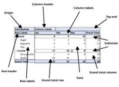
Pivot table defines a map of pivot areas and for each area defines a differential style. The area can be very specific.
Each area has a criteria that are used to determine which cells of the table satisfy the criteria and thus have applied differential style.
The most basic criteria to determine an area is a type, as seen at the image above. There are many others, e.g. only cells that are on a row with a specific pivot field and many others. Full details of all possible criteria can be found in chapter 18.3.1.68 of ECMA-376.
Each cell can be a member of multiple areas. Each area contributes a piece of a style and the final style for the cell is determined by combining the area styles. E.g. If there were two column fields and there were two areas with a specified style: header area of column field 1 should be bold + header area of column field 2 should be red, the combined style would be bold red, because header for each column field references the same cell.
It's possible to select an are in Excel by moving around a table and looking for a change into a small arrow. Once the arrow appears, click once to select whole area and Excel can now apply the style to the selected area.

The header is an area common for all row/column fields. The final style is determined by combined differential styles of all fields for the axis that define style for its header. Use theIXLPivotTable.RowLabels orIXLPivotTable.ColumnLabels to access the pivot field and then use theIXLPivotField.StyleFormat.Header to modify the style of a header of the field for specific axis.
In the example, the both row fields specify the header style and the resulting style is a combination of both styles. Column dimension has only one field and its style modifies the column header, not the row header.

Setup code
privaterecordPastry(stringName,stringCountry,intNumberOfOrders,doubleQuality,stringMonth,DateTime?BakeDate);varpastries=new[]{newPastry("Croissant","India",150,60.2,"Apr",newDateTime(2016,04,21)),newPastry("Croissant","Niger",250,50.42,"May",newDateTime(2016,05,03)),newPastry("Croissant","Botswana",134,22.12,"Jun",newDateTime(2016,06,24)),newPastry("Doughnut","France",250,89.99,"Apr",newDateTime(2017,04,23)),newPastry("Doughnut","Botswana",225,70,"May",newDateTime(2016,05,24)),newPastry("Doughnut","Botswana",210,75.33,"Jun",newDateTime(2016,06,02)),newPastry("Bearclaw","India",134,10.24,"Apr",newDateTime(2016,04,27)),newPastry("Bearclaw","India",184,33.33,"May",newDateTime(2016,05,20)),newPastry("Bearclaw","France",124,25,"Jun",newDateTime(2017,06,05)),newPastry("Danish","India",394,-20.24,"Apr",newDateTime(2017,04,24)),newPastry("Danish","France",190,60,"May",newDateTime(2017,05,08)),newPastry("Danish","France",221,24.76,"Jun",newDateTime(2016,06,21)),newPastry("Scone","India",135,0,"Apr",newDateTime(2017,04,22)),newPastry("SconE","Botswana",122,5.19,"May",newDateTime(2017,05,03)),newPastry("SCONE","France",243,44.2,"Jun",newDateTime(2017,06,14)),};usingvarwb=newXLWorkbook();varws=wb.Worksheets.Add("PastrySalesData");vartable=ws.Cell(1,1).InsertTable(pastries,"PastrySalesData",true);IXLWorksheetptSheet=wb.Worksheets.Add("pivot");IXLPivotTablept=ptSheet.PivotTables.Add("pivot",ptSheet.Cell(1,1),table.AsRange());pt.Theme=XLPivotTableTheme.None;pt.SetRowHeaderCaption("Pastry sales");
IXLPivotFieldnameRowField=pt.RowLabels.Add("Name");IXLPivotFieldmonthRowField=pt.RowLabels.Add("Month");IXLPivotFieldcountryColumnField=pt.ColumnLabels.Add("Country");pt.Values.Add("NumberOfOrders").SetSummaryFormula(XLPivotSummary.Sum);nameRowField.StyleFormats.Header.Style.Fill.BackgroundColor=XLColor.LightBlue;monthRowField.StyleFormats.Header.Style.Font.SetBold().Font.SetFontSize(20);countryColumnField.StyleFormats.Header.Style.Fill.SetBackgroundColor(XLColor.Orange).Font.SetItalic().Font.SetFontSize(12);wb.SaveAs("example-style-pivot-table-headers.xlsx");
Field labels are an area with unique values of the field. Each label area can be separately styled. Styles for different field labels don't combine themselves. Although not apparently visible, each field has a separate area for its labels (see images).
In the example, both row and column fields have a different style for their field labels.
| Example in a compact layout | Example in a tabular layout |
|---|---|
 |  |
Setup code
publicrecordPastry(stringName,stringCountry,intNumberOfOrders,doubleQuality,stringMonth,DateTime?BakeDate);varpastries=new[]{newPastry("Croissant","India",150,60.2,"Apr",newDateTime(2016,04,21)),newPastry("Croissant","Niger",250,50.42,"May",newDateTime(2016,05,03)),newPastry("Croissant","Botswana",134,22.12,"Jun",newDateTime(2016,06,24)),newPastry("Doughnut","France",250,89.99,"Apr",newDateTime(2017,04,23)),newPastry("Doughnut","Botswana",225,70,"May",newDateTime(2016,05,24)),newPastry("Doughnut","Botswana",210,75.33,"Jun",newDateTime(2016,06,02)),newPastry("Bearclaw","India",134,10.24,"Apr",newDateTime(2016,04,27)),newPastry("Bearclaw","India",184,33.33,"May",newDateTime(2016,05,20)),newPastry("Bearclaw","France",124,25,"Jun",newDateTime(2017,06,05)),newPastry("Danish","India",394,-20.24,"Apr",newDateTime(2017,04,24)),newPastry("Danish","France",190,60,"May",newDateTime(2017,05,08)),newPastry("Danish","France",221,24.76,"Jun",newDateTime(2016,06,21)),newPastry("Scone","India",135,0,"Apr",newDateTime(2017,04,22)),newPastry("SconE","Botswana",122,5.19,"May",newDateTime(2017,05,03)),newPastry("SCONE","France",243,44.2,"Jun",newDateTime(2017,06,14)),};usingvarwb=newXLWorkbook();varws=wb.Worksheets.Add("PastrySalesData");vartable=ws.Cell(1,1).InsertTable(pastries,"PastrySalesData",true);IXLWorksheetptSheet=wb.Worksheets.Add("pivot");IXLPivotTablept=ptSheet.PivotTables.Add("pivot",ptSheet.Cell(1,1),table.AsRange());pt.SetRowHeaderCaption("Pastry sales");
pt.Theme=XLPivotTableTheme.None;IXLPivotFieldnameRowField=pt.RowLabels.Add("Name");IXLPivotFieldmonthRowField=pt.RowLabels.Add("Month");IXLPivotFieldcountryColumnField=pt.ColumnLabels.Add("Country");pt.Values.Add("NumberOfOrders").SetSummaryFormula(XLPivotSummary.Sum);nameRowField.StyleFormats.Label.Style.Font.SetBold().Font.SetFontSize(12);monthRowField.StyleFormats.Label.Style.Fill.SetBackgroundColor(XLColor.LightBlue);countryColumnField.StyleFormats.Label.Style.Fill.SetBackgroundColor(XLColor.Orange);wb.SaveAs("example-style-pivot-table-labels.xlsx");
Basic use of data area styling follows an established pattern. It is however the different in a first practical demonstration of dynamic styling criteria from the pivot styling options. You can set style for data values of a data values fields by first getting the pivot field (IXLPivotTable.RowLabels orIXLPivotTable.ColumnLabels) and then by setting theIXLPivotField.StyleFormats.DataValuesFormat.Style property for desired style.Just like other places, when a cell is a part of multiple possible areas, the final style is created by combining all the eligible styles.
Specifying the data value area style doesn't affect styling for field labels or headers.
To be clear, by specifying a style for a row field data area, we mean that criteria to apply the style areall cells that are on a same row as the field label and are in a data area. Calculated number in grand total area are considered a data area. Same thing for the column fields.
That is the reason why in the image without any collapsed rows there aren't any bold data values. No cell with a number is on a row with name row field label. Once the rows for all months of Danish and Doughnut are collapsed, the number are automatically summed up to the respective labels and styling is reapplied. The cells for Danish (B7:E7) and Doughnut (B12:E12) are no longer on a row with label for any month, so there isn't a light blue background. On the other hand, they are not on a row with a label of a Name field and thus have applied style bold. This is a practical demonstration of how the styles of pivot table are applied dynamically (even with different layout form).
| Pivot table without any collapsed rows | Pivot table with collapses rows |
|---|---|
 |  |
| Pivot table without collapsed rows in tabular form | Pivot table with collapsed rows in tabular form |
 |  |
Setup code
publicrecordPastry(stringName,stringCountry,intNumberOfOrders,doubleQuality,stringMonth,DateTime?BakeDate);varpastries=new[]{newPastry("Croissant","India",150,60.2,"Apr",newDateTime(2016,04,21)),newPastry("Croissant","Niger",250,50.42,"May",newDateTime(2016,05,03)),newPastry("Croissant","Botswana",134,22.12,"Jun",newDateTime(2016,06,24)),newPastry("Doughnut","France",250,89.99,"Apr",newDateTime(2017,04,23)),newPastry("Doughnut","Botswana",225,70,"May",newDateTime(2016,05,24)),newPastry("Doughnut","Botswana",210,75.33,"Jun",newDateTime(2016,06,02)),newPastry("Bearclaw","India",134,10.24,"Apr",newDateTime(2016,04,27)),newPastry("Bearclaw","India",184,33.33,"May",newDateTime(2016,05,20)),newPastry("Bearclaw","France",124,25,"Jun",newDateTime(2017,06,05)),newPastry("Danish","India",394,-20.24,"Apr",newDateTime(2017,04,24)),newPastry("Danish","France",190,60,"May",newDateTime(2017,05,08)),newPastry("Danish","France",221,24.76,"Jun",newDateTime(2016,06,21)),newPastry("Scone","India",135,0,"Apr",newDateTime(2017,04,22)),newPastry("SconE","Botswana",122,5.19,"May",newDateTime(2017,05,03)),newPastry("SCONE","France",243,44.2,"Jun",newDateTime(2017,06,14)),};usingvarwb=newXLWorkbook();varws=wb.Worksheets.Add("PastrySalesData");vartable=ws.Cell(1,1).InsertTable(pastries,"PastrySalesData",true);IXLWorksheetptSheet=wb.Worksheets.Add("pivot");IXLPivotTablept=ptSheet.PivotTables.Add("pivot",ptSheet.Cell(1,1),table.AsRange());pt.SetRowHeaderCaption("Pastry sales");
pt.Theme=XLPivotTableTheme.None;IXLPivotFieldnameRowField=pt.RowLabels.Add("Name");IXLPivotFieldmonthRowField=pt.RowLabels.Add("Month");pt.ColumnLabels.Add("Country");pt.Values.Add("NumberOfOrders").SetSummaryFormula(XLPivotSummary.Sum);nameRowField.StyleFormats.DataValuesFormat.Style.Font.Bold=true;monthRowField.StyleFormats.DataValuesFormat.Style.Fill.BackgroundColor=XLColor.LightBlue;wb.SaveAs("example-style-pivot-table-data-values-rows.xlsx");
Subtotals at the top of the group is a function that calculates something from individual rows of the group and displays it next to the field that was used to define the group.In order to use subtotals, pivot table need at least two levels of fields on the chosen axis. Without two levels, there is nothing to group. To enable subtotal, callIXLPivotField.AddSubtotal(XLSubtotalFunction) method with a selected function from theXLSubtotalFunction enum.
Note that styling the top subtotal is same as styling the data values of a row/column field. Styling bottom subtotal requires different API bottom subtotal adds a new cells to the pivot table.
If the field with a top subtotal is collapsed, the calculated subtotal data from the group row are replaced by a sum.
| Data values are from subtotal function | Data values for collapsed rows is a sum |
|---|---|
 |  |
Setup code
publicrecordPastry(stringName,stringCountry,intNumberOfOrders,doubleQuality,stringMonth,DateTime?BakeDate);varpastries=new[]{newPastry("Croissant","India",150,60.2,"Apr",newDateTime(2016,04,21)),newPastry("Croissant","Niger",250,50.42,"May",newDateTime(2016,05,03)),newPastry("Croissant","Botswana",134,22.12,"Jun",newDateTime(2016,06,24)),newPastry("Doughnut","France",250,89.99,"Apr",newDateTime(2017,04,23)),newPastry("Doughnut","Botswana",225,70,"May",newDateTime(2016,05,24)),newPastry("Doughnut","Botswana",210,75.33,"Jun",newDateTime(2016,06,02)),newPastry("Bearclaw","India",134,10.24,"Apr",newDateTime(2016,04,27)),newPastry("Bearclaw","India",184,33.33,"May",newDateTime(2016,05,20)),newPastry("Bearclaw","France",124,25,"Jun",newDateTime(2017,06,05)),newPastry("Danish","India",394,-20.24,"Apr",newDateTime(2017,04,24)),newPastry("Danish","France",190,60,"May",newDateTime(2017,05,08)),newPastry("Danish","France",221,24.76,"Jun",newDateTime(2016,06,21)),newPastry("Scone","India",135,0,"Apr",newDateTime(2017,04,22)),newPastry("SconE","Botswana",122,5.19,"May",newDateTime(2017,05,03)),newPastry("SCONE","France",243,44.2,"Jun",newDateTime(2017,06,14)),};usingvarwb=newXLWorkbook();varws=wb.Worksheets.Add("PastrySalesData");vartable=ws.Cell(1,1).InsertTable(pastries,"PastrySalesData",true);IXLWorksheetptSheet=wb.Worksheets.Add("pivot");IXLPivotTablept=ptSheet.PivotTables.Add("pivot",ptSheet.Cell(1,1),table.AsRange());pt.SetRowHeaderCaption("Pastry sales");
pt.Theme=XLPivotTableTheme.None;pt.SetSubtotals(XLPivotSubtotals.AtTop);IXLPivotFieldnameRowField=pt.RowLabels.Add("Name");pt.RowLabels.Add("Month");pt.ColumnLabels.Add("Country");pt.Values.Add("NumberOfOrders").SetSummaryFormula(XLPivotSummary.Sum);nameRowField.SetSubtotalsAtTop(true)// By default, subtotal is always the top.AddSubtotal(XLSubtotalFunction.Average);nameRowField.StyleFormats.DataValuesFormat.Style.Fill.SetBackgroundColor(XLColor.LightBlue);wb.SaveAs("example-style-pivot-table-subtotal-top.xlsx");
Subtotals require at least two fields in one axis. Once there are multiple fields, you can take any non-last and consider all rows within the field a group. The values of group rows can then summed though a subtotal function and displayed in a subtotal row/column.
To style the subtotal row/column, it is necessary to
- Enable subtotals for pivot table (default value is
XLPivotSubtotals.DoNotShow) by settingIXLPivottable.SetSubtotals(XLPivotSubtotals.AtBottom) - For each non-last row/column field in an axis call
IXLPivotField.SetSubtotalsAtTop(false) - Style the field with subtotal from previous step by modifying the
IXLPivotField.StyleFormats.Subtotal.Style
| Styled subtotal rows without collapsed rows | Styled subtotal with collapsed rows |
|---|---|
 |  |
Setup code
publicrecordPastry(stringName,stringCountry,intNumberOfOrders,doubleQuality,stringMonth,DateTime?BakeDate);varpastries=new[]{newPastry("Croissant","India",150,60.2,"Apr",newDateTime(2016,04,21)),newPastry("Croissant","Niger",250,50.42,"May",newDateTime(2016,05,03)),newPastry("Croissant","Botswana",134,22.12,"Jun",newDateTime(2016,06,24)),newPastry("Doughnut","France",250,89.99,"Apr",newDateTime(2017,04,23)),newPastry("Doughnut","Botswana",225,70,"May",newDateTime(2016,05,24)),newPastry("Doughnut","Botswana",210,75.33,"Jun",newDateTime(2016,06,02)),newPastry("Bearclaw","India",134,10.24,"Apr",newDateTime(2016,04,27)),newPastry("Bearclaw","India",184,33.33,"May",newDateTime(2016,05,20)),newPastry("Bearclaw","France",124,25,"Jun",newDateTime(2017,06,05)),newPastry("Danish","India",394,-20.24,"Apr",newDateTime(2017,04,24)),newPastry("Danish","France",190,60,"May",newDateTime(2017,05,08)),newPastry("Danish","France",221,24.76,"Jun",newDateTime(2016,06,21)),newPastry("Scone","India",135,0,"Apr",newDateTime(2017,04,22)),newPastry("SconE","Botswana",122,5.19,"May",newDateTime(2017,05,03)),newPastry("SCONE","France",243,44.2,"Jun",newDateTime(2017,06,14)),};usingvarwb=newXLWorkbook();varws=wb.Worksheets.Add("PastrySalesData");vartable=ws.Cell(1,1).InsertTable(pastries,"PastrySalesData",true);IXLWorksheetptSheet=wb.Worksheets.Add("pivot");IXLPivotTablept=ptSheet.PivotTables.Add("pivot",ptSheet.Cell(1,1),table.AsRange());ptSheet.SetTabActive();pt.SetRowHeaderCaption("Pastry sales");
pt.Theme=XLPivotTableTheme.None;IXLPivotFieldnameRowField=pt.RowLabels.Add("Name");pt.RowLabels.Add("Month");pt.ColumnLabels.Add("Country");pt.Values.Add("NumberOfOrders").SetSummaryFormula(XLPivotSummary.Sum);pt.SetSubtotals(XLPivotSubtotals.AtBottom);// For bottom subtotal has to be set to AtBottom valuenameRowField.SetSubtotalCaption("Sum of orders").SetSubtotalsAtTop(false)// For bottom subtotal has to be set to false value// .AddSubtotal(XLSubtotalFunction.Average) Bug - subtotal styling works only for default subtotal function (sum), fix per 18.10.2.1;nameRowField.StyleFormats.Subtotal.Style.Fill.SetBackgroundColor(XLColor.LightBlue);wb.SaveAs("example-style-pivot-table-subtotal-bottom.xlsx");
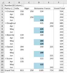
Pivot table styling allows to select a combination of some columns and rows. ClosedXML has an API for that. Take an axis field fromIXLPivotTable.Rowlabels/IXLPivotTable.ColumnLabels and on theIXLPivotStyleFormats property ofIXLPivotField.StyleFormats.DataValuesFormat call a methodAndWith(IXLPivotField, Predicate<object>). The predicate is there to select only certain cells of the field. The value received by the predicate is a value of a cell in the column/row of the field. The methodAndWith is not limited to other axis, see further examples.
In the example, we select only cells that are in
- a row for fieldMonth that has a valueJun orMay and
- a column of a fieldCountry with a valueBotswana

Setup code
publicrecordPastry(stringName,stringCountry,intNumberOfOrders,doubleQuality,stringMonth,DateTime?BakeDate);varpastries=new[]{newPastry("Croissant","India",150,60.2,"Apr",newDateTime(2016,04,21)),newPastry("Croissant","Niger",250,50.42,"May",newDateTime(2016,05,03)),newPastry("Croissant","Botswana",134,22.12,"Jun",newDateTime(2016,06,24)),newPastry("Doughnut","France",250,89.99,"Apr",newDateTime(2017,04,23)),newPastry("Doughnut","Botswana",225,70,"May",newDateTime(2016,05,24)),newPastry("Doughnut","Botswana",210,75.33,"Jun",newDateTime(2016,06,02)),newPastry("Bearclaw","India",134,10.24,"Apr",newDateTime(2016,04,27)),newPastry("Bearclaw","Botswana",184,33.33,"May",newDateTime(2016,05,20)),newPastry("Bearclaw","Botswana",124,25,"Jun",newDateTime(2017,06,05)),newPastry("Danish","India",394,-20.24,"Apr",newDateTime(2017,04,24)),newPastry("Danish","Botswana",190,60,"May",newDateTime(2017,05,08)),newPastry("Danish","France",221,24.76,"Jun",newDateTime(2016,06,21)),newPastry("Scone","India",135,0,"Apr",newDateTime(2017,04,22)),newPastry("SconE","Botswana",122,5.19,"May",newDateTime(2017,05,03)),newPastry("SCONE","France",243,44.2,"Jun",newDateTime(2017,06,14)),};usingvarwb=newXLWorkbook();varws=wb.Worksheets.Add("PastrySalesData");vartable=ws.Cell(1,1).InsertTable(pastries,"PastrySalesData",true);IXLWorksheetptSheet=wb.Worksheets.Add("pivot");IXLPivotTablept=ptSheet.PivotTables.Add("pivot",ptSheet.Cell(1,1),table.AsRange());ptSheet.SetTabActive();pt.SetRowHeaderCaption("Pastry sales");
pt.Theme=XLPivotTableTheme.None;IXLPivotFieldnameRowField=pt.RowLabels.Add("Name");IXLPivotFieldmonthColumnField=pt.RowLabels.Add("Month");IXLPivotFieldcountryColumnField=pt.ColumnLabels.Add("Country");pt.Values.Add("NumberOfOrders").SetSummaryFormula(XLPivotSummary.Sum);nameRowField.StyleFormats.DataValuesFormat.AndWith(countryColumnField, cellValue=>cellValue=="Botswana").AndWith(monthColumnField, cellValue=>cellValue=="May"||cellValue=="Jun").Style.Fill.SetBackgroundColor(XLColor.LightBlue).Font.SetBold(true);wb.SaveAs("example-style-pivot-table-data-value-combination-of-row-and-column.xlsx");
Pivot table can have more than one value at the intersection of a row and a column. To style each value field differently, use theIXLPivotField.StyleFormats.DataValuesFormat.ForValueField method. This method says that only cells laying on the axis field that also belong to the value field should be styled. Conditions for axis field can be further refined by usingAndWith method and its predicate.
In the example, the pivot table has two values: average quality and a total number of orders. we want to highlight cells with a value of qualityat the end of quarter, but keep rest unstylized. We do that by combining row fieldMonth with a value ofJun and further restrict it to only value fieldQuality.

Setup code
publicrecordPastry(stringName,stringCountry,intNumberOfOrders,doubleQuality,stringMonth,DateTime?BakeDate);varpastries=new[]{newPastry("Croissant","India",150,60.2,"Apr",newDateTime(2016,04,21)),newPastry("Croissant","Niger",250,50.42,"May",newDateTime(2016,05,03)),newPastry("Croissant","Botswana",134,22.12,"Jun",newDateTime(2016,06,24)),newPastry("Doughnut","France",250,89.99,"Apr",newDateTime(2017,04,23)),newPastry("Doughnut","Botswana",225,70,"May",newDateTime(2016,05,24)),newPastry("Doughnut","Botswana",210,75.33,"Jun",newDateTime(2016,06,02)),newPastry("Bearclaw","India",134,10.24,"Apr",newDateTime(2016,04,27)),newPastry("Bearclaw","Botswana",184,33.33,"May",newDateTime(2016,05,20)),newPastry("Bearclaw","Botswana",124,25,"Jun",newDateTime(2017,06,05)),newPastry("Danish","India",394,-20.24,"Apr",newDateTime(2017,04,24)),newPastry("Danish","Botswana",190,60,"May",newDateTime(2017,05,08)),newPastry("Danish","France",221,24.76,"Jun",newDateTime(2016,06,21)),newPastry("Scone","India",135,0,"Apr",newDateTime(2017,04,22)),newPastry("SconE","Botswana",122,5.19,"May",newDateTime(2017,05,03)),newPastry("SCONE","France",243,44.2,"Jun",newDateTime(2017,06,14)),};usingvarwb=newXLWorkbook();varws=wb.Worksheets.Add("PastrySalesData");vartable=ws.Cell(1,1).InsertTable(pastries,"PastrySalesData",true);IXLWorksheetptSheet=wb.Worksheets.Add("pivot");IXLPivotTablept=ptSheet.PivotTables.Add("pivot",ptSheet.Cell(1,1),table.AsRange());ptSheet.SetTabActive();pt.SetRowHeaderCaption("Pastry sales");
pt.Theme=XLPivotTableTheme.None;pt.RowLabels.Add("Name");IXLPivotFieldmonthColumnField=pt.RowLabels.Add("Month");pt.ColumnLabels.Add("Country");pt.Values.Add("NumberOfOrders").SetSummaryFormula(XLPivotSummary.Sum);varqualityValueField=pt.Values.Add("Quality").SetSummaryFormula(XLPivotSummary.Average);monthColumnField.StyleFormats.DataValuesFormat.AndWith(monthColumnField, cellValue=>cellValue=="Jun").ForValueField(qualityValueField).Style.Fill.SetBackgroundColor(XLColor.Orange);wb.SaveAs("example-style-pivot-table-combination-axis-field-and-value-field.xlsx");
ClosedXML can modify the style of a row grand total area of a table. Use theXLPivotTable.StyleFormats.RowGrandTotalFormats.ForElement API for that. It's necessary to specify what part of the row grand total should the style be applied. The following example applies
- large font size to the whole row
- red color to the row grand total label area
- green color to the row grand total data area

Setup code
privaterecordPastry(stringName,int?Code,intNumberOfOrders,doubleQuality,stringMonth,DateTime?BakeDate);varpastries=new[]{newPastry("Croissant",101,150,60.2,"Apr",newDateTime(2016,04,21)),newPastry("Croissant",101,250,50.42,"May",newDateTime(2016,05,03)),newPastry("Croissant",101,134,22.12,"Jun",newDateTime(2016,06,24)),newPastry("Doughnut",102,250,89.99,"Apr",newDateTime(2017,04,23)),newPastry("Doughnut",102,225,70,"May",newDateTime(2016,05,24)),newPastry("Doughnut",102,210,75.33,"Jun",newDateTime(2016,06,02)),newPastry("Bearclaw",103,134,10.24,"Apr",newDateTime(2016,04,27)),newPastry("Bearclaw",103,184,33.33,"May",newDateTime(2016,05,20)),newPastry("Bearclaw",103,124,25,"Jun",newDateTime(2017,06,05)),newPastry("Danish",104,394,-20.24,"Apr",newDateTime(2017,04,24)),newPastry("Danish",104,190,60,"May",newDateTime(2017,05,08)),newPastry("Danish",104,221,24.76,"Jun",newDateTime(2016,06,21)),// Deliberately add different casings of same string to ensure pivot table doesn't duplicate it.newPastry("Scone",105,135,0,"Apr",newDateTime(2017,04,22)),newPastry("SconE",105,122,5.19,"May",newDateTime(2017,05,03)),newPastry("SCONE",105,243,44.2,"Jun",newDateTime(2017,06,14)),// For ContainsBlank and integer rows/columns testnewPastry("Scone",null,255,18.4,null,null),};
usingvarwb=newXLWorkbook();varws=wb.Worksheets.Add("PastrySalesData");vartable=ws.Cell(1,1).InsertTable(pastries,"PastrySalesData",true);IXLWorksheetptSheet=wb.Worksheets.Add("pivot");IXLPivotTablept=ptSheet.PivotTables.Add("pivot",ptSheet.Cell(1,1),table.AsRange());pt.Theme=XLPivotTableTheme.None;pt.SetRowHeaderCaption("Pastry sales");pt.RowLabels.Add("Name");pt.ColumnLabels.Add("Month");pt.Values.Add("NumberOfOrders").SetSummaryFormula(XLPivotSummary.Sum);pt.StyleFormats.RowGrandTotalFormats.ForElement(XLPivotStyleFormatElement.All).Style.Font.FontSize=25;pt.StyleFormats.RowGrandTotalFormats.ForElement(XLPivotStyleFormatElement.Label).Style.Fill.BackgroundColor=XLColor.Red;pt.StyleFormats.RowGrandTotalFormats.ForElement(XLPivotStyleFormatElement.Data).Style.Fill.BackgroundColor=XLColor.Green;wb.SaveAs("example-style-pivot-table-grand-total.xlsx");
Setup code
- How do I deliver an Excel file in ASP.NET?
- Does it support Excel 2003 and prior formats (.xls)?
- How can I insert an image?
- Text with numbers are getting converted to numbers, what's up with that?
- How do I get the result of a formula?
- Data Types
- Creating Multiple Worksheets
- Organizing Sheets
- Loading and Modifying Files
- Using Lambda Expressions
- Cell Values
- Workbook Properties
- Using Formulas
- Evaluating Formulas
- Creating Rows And Columns Outlines
- Hide Unhide Rows And Columns
- Freeze Panes
- Copying Worksheets
- Using Hyperlinks
- Data Validation
- Hide Worksheets
- Sheet Protection
- Tab Colors
- Conditional Formatting
- Pivot Table example
- Sparklines
- Copying IEnumerable Collections
- Inserting Data
- Inserting Tables
- Adding DataTable as Worksheet
- Adding DataSet
- Styles - Alignment
- Styles - Border
- Styles - Fill
- Styles - Font
- Styles - NumberFormat
- NumberFormatId Lookup Table
- Style Worksheet
- Style Rows and Columns
- Using Default Styles
- Using Colors
- ClosedXML Predefined Colors
- Excel Indexed Colors
- Using Rich Text
- Using Phonetics
- Defining Ranges
- Merging Cells
- Clearing Ranges
- Deleting Ranges
- Multiple Ranges
- Shifting Ranges
- Transpose Ranges
- Named Ranges
- Accessing Named Ranges
- Copying Ranges
- Using Tables
- Sorting Data
- Selecting Cells and Ranges
- Row Height and Styles
- Selecting Rows
- Inserting Rows
- Inserting and Deleting Rows
- Adjust Row Height and Column Width to Contents
- Row Cells
- Column Width and Styles
- Selecting Columns
- Inserting Columns
- Inserting and Deleting Columns
- Adjust Row Height and Column Width to Contents
- Column Cells
- Pages Tab
- Paper Size Lookup Table
- Margins Tab
- Headers and Footers Tab
- Sheet Tab
- Print Areas and Page Breaks