
Mapping habitat connectivity with geohabnet
KrishnaKeshav(krishnakeshav.pes@gmail.com)
01 November, 2025
Source:vignettes/articles/analysis.Rmdanalysis.RmdAbstract
Habitat connectivity can be used to analyse the potential spread ofplant pathogen, pest, or any habitat-dependent species. Habitatconnectivity of a species depends on the habitat availability (e.g.,host availability for plant pests or pollinators or availability offavorable climate for plant species), and probability of movement of aspecies between habitat locations. Ingeohabnet, habitatconnectivity indicates the importance of a habitat location infacilitating the spread of a species across a geographic region,relative to other locations in the same landscape. For plant pathogensand pests, the spatial distribution of host availability plays a crucialrole for defining habitat availability and the establishment of the pestspecies. Locations with abundant habitats (e.g., plant hosts) may play aminor role in species spread if they are isolated. Yet, a location withlimited habitat may play a major role in the spread of a species if itacts as a bridge between regions that would otherwise be separated.geohabnet(Keshav, Plex, and Garrett2025) provides the R-user community with a network-based approachto estimate habitat connectivity across the world. This package supportsup to 10 parameters that has potential to influence habitat or landscapeconnectivity. The implementation ofgeohabnet(Keshav, Plex, and Garrett 2025) expands thecropland connectivity method for plant pathogens proposed by(Xing et al. 2020) to a general way ofcalculating habitat connectivity for any species. The network-basedframework is the same as the one proposed by(Xing et al. 2020). However,geohabnetprovides more flexibility to users to modify any parameter values inthis framework.
Although this article focuses on the use ofgeohabnet(Keshav et al. 2023), it is useful to know forinterested developers that package design is inspired from widely usedConfiguration-based design in software development(Majors 2022),(Nash andDeMore 2009); and(Allaire 2023)provides a text based interface to control the parameters values forrisk analysis in this context.
The primary objective of this vignette is to help user beingfamiliarized withgeohabnet(Keshav etal. 2023), list its capabilities and get an intuition behindthem. It also describes the implementation of the main functions ingeohabnet to support this intuition. Throughout the article, wewill be citing external sites and resources, which are relevant for theuse of this package.
Pre-requisites
Definitions
Raster - Raster is a digital encoding representation ofgeographic information as a grid of cells or pixels, where each cellcontains a value representing a specific property or attribute of alocation. Some details of a raster data include spatial resolution,dimensions, or geographic extent, which are useful in identification andprocessing. Here, we use raster to represent maps.
TIFF(Tag Image File Format) is a type of file that storesgeographic information in the form of raster.(Keshav et al. 2023) has been tested using.tif and.nc files but it would be able to handle anyraster type of file supported by the R packageterra(Hijmans 2023) .
Data sets
For estimating habitat connectivity for understanding the spread ofplant pathogens or pests, we use cropland density or host availabilityaround the world as a proxy for habitat availability (this assumptioncan be complemented with species-specific environmental suitability fora better proxy of habitat availability). We use publicly availablesources to obtain crop distribution in the form of raster layers.
CROPGRIDS(Tang FHM 2024)
EARTHSTAT(Monfreda, Ramankutty, and Foley2008)
MapSpam(2010, 2017)(International Food PolicyResearch Institute 2019)
CroplandCROS(Service 2025)
GBIF(GBIF 2025)
geodata provides a set of APIs to access the EARTHSTAT andMapSPAM datasets directly in R (see code below).
The raster layers from the data sources listed above may need sometransformation before using them in(Keshav etal. 2023). A valid raster layer to be used is one that its entryvalues of each pixel range from 0 (no habitat available) to 1 (habitatis available in the entirety of the pixel). For example, data layers ofcropland fraction from EARTHSTAT can be directly provided to functionswithout the need to re-scale its entries. However, data layers ofharvested area from CROPGRIDS will need re-scaling the values of eachgrid cell in the raster (see an example of how to do this below).
For visualization and plots,geohabnet usesrnaturalearthrnaturalearth.
Quick Start
Meta information
- Package information -https://garrettlab.github.io/HabitatConnectivity/
- CRAN site -https://CRAN.R-project.org/package=geohabnet
- Source code -https://github.com/GarrettLab/HabitatConnectivity/tree/main/geohabnet/
- Report issues -https://github.com/GarrettLab/CroplandConnectivity/issues/
- Garrett lab website -https://www.garrettlab.com/
Installation and loading
Installinggeohabnet will automatically install itsdependencies on other R packages. See the list of dependencies usingdesc::desc(package = "geohabnet")
if(!require("devtools")){install.packages("devtools")}if(!require("geohabnet")){utils::install.packages("geohabnet")}Alternatively, you can install the development version ofgeohabnet from GitHub repository.
library("devtools")#> Loading required package: usethisif(!require("geohabnet")){install_github("GarrettLab/HabitatConnectivity", subdir="geohabnet")}#> Loading required package: geohabnetEither way, now you can loadgeohabnet in R asfollows:
At any point, you can access the help page using the following
?geohabnet# For description of the package# and?geohabnet::msean# For documentation of a function (in this case, the msean function)Habitat connectivity analysis based on default parameters
The section below illustrate how the habitat connectivity analysiscan be conducted using the default set of values for the supportedparameters. For this example, we use the raster layer for avocadoharvested area from CROPGRIDS(Tang FHM2024) as a real-world case study for the habitat connectivity ofavocado-specific pathogens. This example would run the analysis onglobal geographical extent relatively quickly since the crop presencearound the world is relatively low.
For the purposes of demonstration, the code below sets the hostparameter programatically or directly in RStudio. Alternatively, theparameters can be fed viaparameters.yaml in an interactiveway using either the path or settingiwindow = TRUE for thewindows prompt inset_parameters()
Running your first habitat connectivity analysis
If you are also replicating this example, please first download theavocado layer from CROPGRIDS and put it in the folder you are currentlyworking. Note that we are downloading the raster layer for hostavailability (or habitat availability) manually from CROPGRIDS. However,an alternative option is getting the data layer directly in RStudiousing thegeodata package (depending on whether it is downor not). At the time, we created this vignettegeodata wasnot working on our local machine but the R code to do so isprovided.
#if (!require(geodata))# install.packages("geodata")#avocado_sp <- geodata::crop_monfreda(crop = "avocado", var = "area_ha", path = tools::R_user_dir("geohabnet", which = "config"))library(terra)#> terra 1.8.50#avocado_rast_input <- system.file("CROPGRIDSv1.08_avocado.nc", package = "geohabnet", mustWork = TRUE)avocado_sp<-rast("CROPGRIDSv1.08_avocado.nc")cell.area<-(0.05*111111)*(0.05*111111)/10000#area in heactaresavocado_sp<-avocado_sp$harvarea/cell.area#area in hectaresvalues(avocado_sp)<-ifelse(values(avocado_sp)>0,values(avocado_sp),NaN)avocado_sp<-aggregate(avocado_sp, fact=2, fun="mean", na.rm=TRUE)#> |---------|---------|---------|---------|=========================================writeRaster(avocado_sp,"avocado_density.tif", overwrite=TRUE)Note that, apart from getting the raster in R, we are also scalingthe entry values of each grid cell in the raster layer, from harvestedarea in hectares to avocado cropland fraction. We are aggregating thisraster layer to reduce computational cost when running the analysis (forillustrative purposes only, you may not need to do this for your owndata set). We are also saving the new avocado area fraction as a newraster layer in our local machines.
Setting values in a function
Now let’s visualize how the avocado area fraction looks like. Theinternal implementation and program deals with object ofterra(Hijmans 2023) andigraph(Csardi and Nepusz2006) . The primary object is of typeSpatRasterfromterra.
In the example below, we will use the same spatial raster obtainedfor avocado. First, it shows the properties of the raster layer, whichwe will learn about them below. [gplot()] quickly shows the content ofraster layer.
avocado_sp#> class : SpatRaster#> dimensions : 1800, 3600, 1 (nrow, ncol, nlyr)#> resolution : 0.1, 0.1 (x, y)#> extent : -180, 180, -90, 90 (xmin, xmax, ymin, ymax)#> coord. ref. :#> source(s) : memory#> name : harvarea#> min value : 3.268422e-06#> max value : 1.700697e-01gplot(avocado_sp)
Now that we have a raster object in R, this raster layer can be usedas the input in themsean function (one of the mainfunctions ofgeohabnet) to produce your first habitatconnectivity analysis. In this case, we are providing input for thealways-required parameter -rast and keeping the default valuesfor the other parameters supported by this function (for now). Runningthe example below usually takes 5-10 minutes depending on the processingpower of your machine.
geo_net<-msean(avocado_sp)#> |---------|---------|---------|---------|=====#> Warning: [+] CRS do not match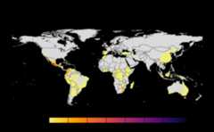
#> |---------|---------|---------|---------|======#> Warning: [+] CRS do not match#> |---------|---------|---------|---------|==========#> Warning: [+] CRS do not match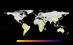
#> |---------|---------|---------|---------|====#> Warning: [+] CRS do not match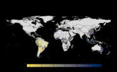
Many, many congratulations! You have just generated a fullsensitivity analysis of habitat connectivity for avocado-specificpathogens and pests. Take a minute to appreciate the beauty of our threeoutcome maps: the map of mean habitat connectivity, the map of variancehabitat connectivity, and the map of the difference between them.
Now let’s dive a little bit on the nitty-gritty details. The functionmsean is very similar tosean except thatmsean() is able to produce the maps above. They also returndifferent S4 objects: aGeoNetwork object is produced bymsean, whilesean produces aGeoRasters object. The results should be interpreted inaccordance to the values of other parameters that have factored asarguments tosean. Run ?sean to see all the supportedparameters. For now, let’s focus on some parameters you might want tochange.
rast -spatRaster. Represents the map ofhabitat availability in a geographical area. In our example above, thisis
avocado_sp, the unique parameter that was provided tomsean.geoscale -Vector. Refers to the geographicalcoordinates in the form of c(Xmin, Xmax, Ymin, Ymax).
global -Logical. When set as TRUE,geoscale is ignored.
You can get the geographical scales used in a global habitatconnectivity analysis (like the one above) by running
global_scales()#> $east#> [1] -24 180 -58 60#>#> $west#> [1] -140 -34 -58 60It is not highly recommended to change the default value forglobal scales used for a global connectivity analysis since it has beenfinalized after several tries. However, if you need to change the globalscale for an advanced use, you can set different global geographicscales using the following
#set_global_scales(list(east = c(-24, 180, -58, 60), west = c(-140, -34, -58, 60)))
thresholds- Numeric.
mseansupports two types of thresholds:host density andlinkweights represented byhd_threshold andlink_threshold, respectively. The former threshold(host density threshold or habitat availability threshold) excludes fromthe habitat connectivity analysis all values in aggregated raster layerbelow this threshold. The latter threshold (link weight threshold)excludes from the habitat connectivity analysis all entry values in theadjacency matrix that are below this threshold. Entries in the adjacencymatrix (or link weights in its corresponding network) are the product ofhabitat availability and the relative likelihood of dispersal betweeneach pair of locations in the selected region.resolution - Numeric. This is a spatial aggregationvalue. In the context ofSpatRaster, this parameter is thenumber of pixels that are aggregated to produce a new finer/coarserversion raster data layer. Default is
reso()#> [1] 12Outcomes -
mseancalculates, produces, and plotsthree maps of habitat connectivity in a region, which are the sameoutcomes produced bysensitivity_analysis()(the other mainfunction ofgeohabnet). An alternative issean()which can be called to obtain the results from thefunction call and has no side effects.
Using configuration
More parameters are available under configuration and thus morecontrol over the analysis. The configuration file name isparameters.yaml, currently supporting up to 10 parameters.The intuition behind this methodology is to provide a basic interfacefor setting new values. The snippet below describes the basic usage ofconfiguration.
Get the initial configuration file. By default this function willsave the file in temporary directorytempdir(), however werecommend saving to path where program will have write permissions.Usingiwindow = TRUE will prompt a selection window to saveconfig file.
config_file<-get_parameters(out_path=tempdir())config_file#> [1] "/var/folders/r5/zggvft9d3yn5kh51wqp78rd00000gn/T//RtmphRPeWc/parameters.yaml"The file should look something like this -

The values must be modified without modifying the structure. Theorder don’t matter for the program. The new values in the configurationmust be fed to the workflow. For the purposes of demonstration, the codebelow sets the host parameter programmitically. The parameters can befed viaparameters.yaml in an interactive way as well usingeither the path or settingiwindow = TRUE for the windowsprompt inset_parameters()
if(!require("geodata")){install.packages("geodata")}#> Loading required package: geodatapath_to_avo<-"avocado_density.tif"#terra::sources(avocado_sp)params_file<-geohabnet::get_parameters()if(!require(yaml))install.packages("yaml")#> Loading required package: yamlparams_yaml<-yaml::yaml.load_file(params_file)params_yaml$default$`CCRI parameters`$Host<-path_to_avoyaml::write_yaml(params_yaml,params_file)geohabnet::set_parameters(params_file)#> [1] TRUE#using iwindow = true will prompt a selection window to choose config file.get_parameters() was only to fetch the initialparameters. While you can, it is not required to re-fetch if theparameters has not been modified in the configuration. Modify the valueand feed it to workflow usingset_parameters().
Parameters
Hosts
The library supports a spatial raster file (e.g. TIFF). The casestudies were done on crop data from Monfreda(Monfreda, Ramankutty, and Foley 2008) andMapspam(International Food Policy ResearchInstitute 2019) which is available viageodatapackage(geodata2025?)
results<-sensitivity_analysis()#> Warning in max(wv, na.rm = TRUE): no non-missing arguments to max; returning#> -Inf#> Warning in max(wv, na.rm = TRUE): no non-missing arguments to max; returning#> -Inf#> Warning in max(wv, na.rm = TRUE): no non-missing arguments to max; returning#> -Inf#> Warning in max(wv, na.rm = TRUE): no non-missing arguments to max; returning#> -Inf#> Warning in max(wv, na.rm = TRUE): no non-missing arguments to max; returning#> -Inf#> Warning in max(wv, na.rm = TRUE): no non-missing arguments to max; returning#> -Inf#> Warning in max(wv, na.rm = TRUE): no non-missing arguments to max; returning#> -Inf#> Warning in max(wv, na.rm = TRUE): no non-missing arguments to max; returning#> -Inf#> Warning in max(wv, na.rm = TRUE): no non-missing arguments to max; returning#> -Inf#> Warning in max(wv, na.rm = TRUE): no non-missing arguments to max; returning#> -Inf#> Warning in max(wv, na.rm = TRUE): no non-missing arguments to max; returning#> -Inf#> Warning in max(wv, na.rm = TRUE): no non-missing arguments to max; returning#> -Inf#> Warning in max(wv, na.rm = TRUE): no non-missing arguments to max; returning#> -Inf#> Warning in max(wv, na.rm = TRUE): no non-missing arguments to max; returning#> -Inf#> Warning in max(wv, na.rm = TRUE): no non-missing arguments to max; returning#> -Inf#> Warning in max(wv, na.rm = TRUE): no non-missing arguments to max; returning#> -Inf#> Warning in max(wv, na.rm = TRUE): no non-missing arguments to max; returning#> -Inf#> Warning in max(wv, na.rm = TRUE): no non-missing arguments to max; returning#> -Inf#> Warning in max(wv, na.rm = TRUE): no non-missing arguments to max; returning#> -Inf#> Warning in max(wv, na.rm = TRUE): no non-missing arguments to max; returning#> -Inf#> Warning in max(wv, na.rm = TRUE): no non-missing arguments to max; returning#> -Inf#> Warning in max(wv, na.rm = TRUE): no non-missing arguments to max; returning#> -Inf#> Warning in max(wv, na.rm = TRUE): no non-missing arguments to max; returning#> -Inf#> Warning in max(wv, na.rm = TRUE): no non-missing arguments to max; returning#> -Inf#> Warning in max(wv, na.rm = TRUE): no non-missing arguments to max; returning#> -Inf#> Warning in max(wv, na.rm = TRUE): no non-missing arguments to max; returning#> -Inf#> Warning in max(wv, na.rm = TRUE): no non-missing arguments to max; returning#> -Inf#> Warning in max(wv, na.rm = TRUE): no non-missing arguments to max; returning#> -Inf#> Warning in max(wv, na.rm = TRUE): no non-missing arguments to max; returning#> -Inf#> Warning in max(wv, na.rm = TRUE): no non-missing arguments to max; returning#> -Inf#> |---------|---------|---------|---------|====#> Warning: [+] CRS do not match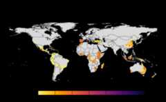
#> |---------|---------|---------|---------|======#> Warning: [+] CRS do not match#> |---------|---------|---------|---------|==========#> Warning: [+] CRS do not match
#> |---------|---------|---------|---------|====#> Warning: [+] CRS do not match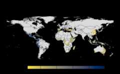
Thresholds
Thresholds are used to select subset of values from theSpatRaster on which the operations are applied. It directlyeffects the connectivity and gives a sense of sensitivity in thenetwork. The intermediate goal is to produce a adjacency graph whichessentially determines the connectivity. Cells which doesn’t meet thethreshold are removed from the consideration by dispersal models.
risk_indexes<-msean(avocado_sp, global=FALSE, hd_threshold=0.0001, link_threshold=0.001)#> Warning in max(wv, na.rm = TRUE): no non-missing arguments to max; returning#> -Inf#> Warning in max(wv, na.rm = TRUE): no non-missing arguments to max; returning#> -Inf#> Warning in max(wv, na.rm = TRUE): no non-missing arguments to max; returning#> -Inf#> Warning in max(wv, na.rm = TRUE): no non-missing arguments to max; returning#> -Inf#> Warning in max(wv, na.rm = TRUE): no non-missing arguments to max; returning#> -Inf#> Warning in max(wv, na.rm = TRUE): no non-missing arguments to max; returning#> -Inf#> Warning in max(wv, na.rm = TRUE): no non-missing arguments to max; returning#> -Inf#> Warning in max(wv, na.rm = TRUE): no non-missing arguments to max; returning#> -Inf#> |---------|---------|---------|---------|==#> Warning: [+] CRS do not match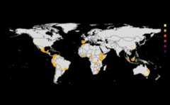
#> |---------|---------|---------|---------|==#> Warning: [+] CRS do not match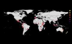
#> |---------|---------|---------|---------|==#> Warning: [+] CRS do not match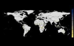
Density Thresholds
host density threshold. The host density threshold is the minimumcropland proportion in the grid cells (or locations) that will beincluded in the analysis. This parameter is calledHostDensityThreshold and supports a list of values between0 and 1. Before running the sensitivity_analysis() function, check thatthe values for the host density threshold are smaller than the maximumhost density in the map to prevent errors. The values are rounded off to5 decimal points.
Link Thresholds
Based on the information on host distribution and dispersal kernels,adjacency matrices are created, where entries are the likelihood ofpathogen movement between locations. Then, adjacency matrices areconverted into graph objects to perform a network analysis, where theentries in the adjacency matrices now are the weight of the links of thenetwork.
Choosing link weight thresholds helps to focus the analysis on themore likely pathogen dispersal in the landscape.
Like what you did with the host density threshold, you can provide alist of positive values toLinkThreshold. Before runningthe sensitivity_analysis() function, check that the values for the linkweight threshold are smaller than the maximum link weight in the networkto prevent errors.
Aggregation
Aggregation strategy refers to the function used to create a new mapof host density with a lower resolution (larger cells). Reducing thespatial resolution helps to reduce the computational power needed to runthe analysis.
If AggregationStrategy: [sum], then the sum of the croplandproportion of all initially small grids within a large grid is dividedby the total number of initially small grids within that largegrid.
If AggregationStrategy: [mean], then the sum of the croplandproportion of all initially small grids within a large grid is dividedby the total number of initially small grids containing only land (wheresmall grids with water are excluded) within that large grid.
By default, analysis is run on both but can be opted out from one. Ifonly one method is used, then the difference map is skipped from theoutcome.
Distance methods
For each pair of locations in the host map with values greater thanthe host density threshold, the sensitivity_analysis() function willcalculate the physical distances and use them to calculate the relativelikelihood of pathogen movement between locations based on theirpairwise geographical proximity.
There are two different options to calculate the distance betweenlocations.
· Vincenty ellipsoid distance
This option is highly accurate but more computationallyexpensive.
· Geodesic distance
This option is less computationally expensive and less accurate thanthe option above.
You can set the distance option either asDistanceStrategy:“vincentyEllipsoid” orDistanceStrategy: “geodesic”. Oneof these options should be used as input to run the analysis. Check forsupported methods in analysis by runningdist_methods() inthe console.
dist_methods()#> [1] "geodesic" "vincentyellipsoid"Resolution
The aggregation factor or granularity is the number of small gridcells that are aggregated into larger grid cells in each direction(horizontally and vertically). The finest value is 1 which can requireanalysis to run up to hours because of large number of cells inSpatRaster . The resolution is also used in calculation ofvariance while dis-aggregating the risk indices into coarser resolutionfor producing maps.
If not provided, the defaulted value is selected fromreso()
Metrics
See available metrics using
supported_metrics()#> [1] "betweeness" "node_strength"#> [3] "sum_of_nearest_neighbors" "eigenvector_centrality"#> [5] "closeness" "degree"#> [7] "page_rank"Metrics corresponding to dispersal models are applied to distancematrix with specified weights. The weights must be specified in % andsum of all the weights should be equal to 100. We use functions from(Csardi and Nepusz 2006) to calculatemetrics for each dispersal model. The 2 dispersal models that areapplied to parametersinverse power law andnegativeexponential. More formally, metrics are way to determineconnectivity among nodes in a network.
In a graph functions of(Csardi and Nepusz2006), the links are interpreted as distances. However, in thecontext of habitat connectivity, the network is adapted to interpretlinks as weights which means that the likelihood of pathogen spread islower if the distance is larger.$$L = \frac{1}{W}, \\W' = \sum_{i=1}^{N} \max(W - W_i)$$
L is link weights and W is the original weights in an undirectedgraph. W’ is the transformed weight vector for calculating networkcentrality.
Geographical Extent
Geographical extent is a subset of world map defined by coordinatereference system. The corresponding parameter to set the area insean() andsensitivity_analyis() isgeoscale andGeoExtent respectively. Defaultsetting isglobal = TRUE which will ignore the value ofgeoscale. This will consider taking the world map intoaccount using values fromglobal_scales() . For non-globalanalysis, either setglobal = FALSE with or without thesettinggeoscale. By default,geoscale will beextracted from the extents from the input SpatRaster. We recommend usingEPSG:4326 as coordinate reference system because the functions have beentested on it.
Using function

#> Warning: [+] CRS do not match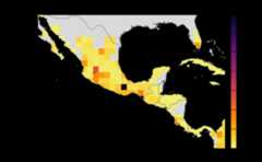
#> Warning: [+] CRS do not match
Using config
Set
Global = FALSEandCustomExt = [-115, -75, 5, 32]. The initialparameters.yamlalready contains this value which would runin combination with other parameters.
When provided withgeoscale, program will take thesubset of provided raster (data-set of a crop). The workflow will applygraph operations and network connectivity only to the subset.
Outputs
By default, 3 maps are produced for each analysis.sean() also returns risk indices without maps which can,then be fed toconnectivity() . This flexibility issupposed to allow users to use the risk indices for their purposes oruse our function to produce maps with further different parameters.
In a code below, after obtaining results, the maps are produced. Inorder to calculate variance, cells ofSpatRaster areextended to coarser value usingres parameter. Settingmaps = FALSE will suppress the calculation of outputs.
sean(avocado) +.connectivity(georast) isequivalent tosensitivity_analysis() ormsean() which produces maps as side effect. The userfunction equivalent is connectivity() which accepts primitives typesinstead of S4 class.
final<-msean(avocado_sp, link_threshold=0.0001, hd_threshold=0.0025)#> Warning in max(wv, na.rm = TRUE): no non-missing arguments to max; returning#> -Inf#> Warning in max(wv, na.rm = TRUE): no non-missing arguments to max; returning#> -Inf#> Warning in max(wv, na.rm = TRUE): no non-missing arguments to max; returning#> -Inf#> Warning in max(wv, na.rm = TRUE): no non-missing arguments to max; returning#> -Inf#> Warning in max(wv, na.rm = TRUE): no non-missing arguments to max; returning#> -Inf#> Warning in max(wv, na.rm = TRUE): no non-missing arguments to max; returning#> -Inf#> Warning in max(wv, na.rm = TRUE): no non-missing arguments to max; returning#> -Inf#> Warning in max(wv, na.rm = TRUE): no non-missing arguments to max; returning#> -Inf#> Warning in max(wv, na.rm = TRUE): no non-missing arguments to max; returning#> -Inf#> Warning in max(wv, na.rm = TRUE): no non-missing arguments to max; returning#> -Inf#> Warning in max(wv, na.rm = TRUE): no non-missing arguments to max; returning#> -Inf#> Warning in max(wv, na.rm = TRUE): no non-missing arguments to max; returning#> -Inf#> Warning in max(wv, na.rm = TRUE): no non-missing arguments to max; returning#> -Inf#> Warning in max(wv, na.rm = TRUE): no non-missing arguments to max; returning#> -Inf#> Warning in max(wv, na.rm = TRUE): no non-missing arguments to max; returning#> -Inf#> |---------|---------|---------|---------|====#> Warning: [+] CRS do not match
#> |---------|---------|---------|---------|======#> Warning: [+] CRS do not match#> |---------|---------|---------|---------|==========#> Warning: [+] CRS do not match
#> |---------|---------|---------|---------|====#> Warning: [+] CRS do not match
# checkout the type of an objectclass(final)#> [1] "GeoNetwork"#> attr(,"package")#> [1] "geohabnet"Based on the result obtained from last cell, let’s navigate theobject final object. You would have noticed the maps as a side effectand that’s really the whole point. See the result summary by simplycalling thefinal object and navigate using the standard S4classes approach.
final#> class : GeoNetwork#> habitat density : 98 , 267 (nrow, ncol) SpatRaster#> mean : /var/folders/r5/zggvft9d3yn5kh51wqp78rd00000gn/T//RtmphRPeWc/plots/mean_20251101192717060378.tif#> mean raster : 1176 , 3204 (nrow, ncol)#> variance : /var/folders/r5/zggvft9d3yn5kh51wqp78rd00000gn/T//RtmphRPeWc/plots/variance_20251101192718031884.tif#> variance raster : 1176 , 3204 (nrow, ncol)#> difference : /var/folders/r5/zggvft9d3yn5kh51wqp78rd00000gn/T//RtmphRPeWc/plots/difference_2025110119271871457.tif#> difference raster : 1176 , 3204 (nrow, ncol)The final operations are performed risk indices and on the 3 resultsthat are produced -
Mean
A mean of all the
SpatRastersresulting from combinationof parameter values. The values in cells are added across all theindices and divided by number of indices. It represents the connectivitybased on host density in the given area.Navigating the resulting object -
gplot(final@me_rast)Variance
Uses
stats::varon risk indices, subset is extracted forprovided scale and finally pixels are dis-aggregated usingfactor =resolution value in original parameter to from previous step.gplot(final@var_rast)Difference
If both the aggregation methods (sum and mean) is selected,then difference is calculated between the rank of matrices which areessentially numeric cells of risk indices of typeSpatRaster.The result is dis-aggregated in the same way as previous step.
gplot(final@diff_rast)
The path to saved raster can be accessed using the ‘type_out’ slot.Additionally, access the risk indices and it’s corresponding adjacencyare further accessible within slots in theGeoNetworkclass.
# checkout the resultsfinal@rasters#> class : GeoRasters#> global : TRUE#> globals : 1# global is TRUE because we original set the global analysis# thus, we will have set of 2 risk indices, eastern and wetern hemispherefinal@rasters$global_rast#> [[1]]#> class : GlobalRast#> east : 14#> west : 14# Number of elements from above determines the the number of parameter values provided# To access the adjacency matrix,final@rasters$global_rast[[1]]$east[[1]]# this is also s4 class 'GeoModel'#> class : GeoModel#> adjacency matrix : 1 , 1 (nrow, ncol)#> risk index : 98 , 170 (nrow, ncol)Checkout the adjacency matrices by running the code below -
# replace the indexing with any arbitary index,# uncomment line below to see the results.#final@rasters$global_rast[[1]]$east[[1]]$amatrixSetpmean, pvar, pdiff toFALSE to skip the any ofthe calculation inconnectivity() to skip this calculation.Insean() orsensitivity_analysis(), setmap = FALSE to skip the generation of maps as an outcome.In case of global analysis, result of eastern and western geographicextents are merged usingterra::merge() . The outcome ofeach of the operation are saved in the new directoryplotsunder the specified path inOutDir with nameopt_datetime.tif, whereopt is one of the abovesuffixed by datetime of the file created. If theoutdir isempty, the value is defaulted totempdir() . This appliesto corresponding parameteroutdir in all the functions.
Computing
To understand the motivation behind implementation, let’s analyze thecomplexity. Since link and host density threshold is a list, let thesize be N. For the kernel models, let’s represent metrics and dispersalcoefficients as x and 4 reprectively. The overall complexity turns outto be. Here, we have assumed the availability of host density. Although, thecrop data is fetched in parallel to minimize the download time.Considering, the complexity will now be.We discount the complexity of graph operations like those of centralityscores because we haven’t attempted to optimize these operations. We tryto optimize the performance through scaling which is fixed problem size,but increasing parallelism.
The operations are compute intensive. Therun_mseansnippet underHosts used up to 8.3GB of memorywhich was 81% of the memory allotted to RStudio. For the most part, theimplementation has focused on performance over efficient memoryusage.
This Package applies mechanisms such as vectorization and foreach toimprove the performance and efficiency. The workflow has several partsrunning independently. There are independent functions which performsoperations such adjacency matrix and or aggregation. This created anopportunity for task level parallelism in running functions withingeohabnet. Each combination of parameters can be run independently andin parallel through most of the parts using future mechanism. Theimplementation supports workflow acceleration using(Bengtsson 2021a, 2021b) . It is also importantto note that we use SpatRaster object throughout the computation.SpatRaster is an external pointer in C++ rather than an R object andthus adds overhead of conversion, neutralizing the performancegains.