


1. Introduction
The twenty-five years following the discovery of the first indisputable brown dwarf,Gliese 229 B (Oppenheimer et al.1995), have seen a flowering of this field. Thousands of brown dwarfshave been discovered and characterized by spectroscopy and photometry (Joergens2014). Dynamical masses andparallaxes have been measured for many objects and a wealth of trends uncovered(e.g., Dupuy & Liu2017; Bestet al.2020). In addition, young,self-luminous planets have been discovered and characterized (e.g., Marois et al.2008).
Most of these objects have been characterized with the help of forward modeling inwhich modelers construct hundreds to thousands of “grid models.” The models, relyingupon fundamental physical processes, predict spectral and evolutionarycharacteristics of brown dwarfs for given choices of intrinsic parameters, such asmass, age, and bulk composition. This approach typically relies upon bothone-dimensional radiative-convective equilibrium atmosphere models and coupledinterior and evolution models. The atmosphere models aim to capture the keyinfluences on substellar atmospheres, including chemistry, dynamics, and cloudprocesses in order to compute the vertical structure of an atmosphere whichconservatively transports energy upwards from the deep interior. Evolution modelsapply the rate of energy loss through the atmosphere as a boundary condition inorder to compute the evolution of radius and luminosity through time.
Such a forward modeling approach provides a self-consistent solution for the coupledproblem of understanding both atmospheric and interior physical processes. By makingpredictions, models inform observers of interesting observational tests and connectobservable properties, including luminosity and the spectral energy distribution, tothe physical properties of the object, including mass and age. Grids of models arealso essential for motivating and planning new observations. A non-exhaustive listof forward model grids includes those of Burrows et al. (1997), Baraffe et al. (2003), Saumon & Marley (2008), Allard et al. (2014), Baraffe et al. (2015), Malik et al. (2017), and Phillips et al. (2020).
The older models in the literature are generally out of date as our knowledge ofmolecular opacities, most notably water and methane, which are important absorbersin substellar atmospheres, has progressed substantially over the intervening years.Several of the more recent grid models use updated opacities but are generally notcoupled with self-consistent evolution calculations, and thus do not provide aself-consistent evolutionary-atmospheric modeling framework, a notable exceptionbeing Phillips et al. (2020) andthe ATMO2020 grid. Here we also provide such a framework, presenting coupledatmospheric structure and evolution models for a variety of atmospheric chemicalassumptions. This effort is the first in an expected series of papers, each lookingat additional model complexities, including disequilibrium chemistry, clouds, and soon. Independent modeling efforts, such as our own and that of Phillips et al. (2020), are crucial forcross-checking the importance of various physical and chemical assumptions and foroverall self-consistency. Thus, we view the Sonora and ATMO2020 model sets to behighly complementary. Further comparisons to some of the other model sets arediscussed in Section2.6.
In the past few years “retrieval methods,” originally developed to study planetaryatmospheres, have been applied to brown dwarfs (e.g., Line et al.2015,2017; Kitzmann et al.2020; Piette & Madhusudhan2020; Burningham et al.2021) in order to understand the constraints onmass, luminosity, composition, radius, and other characteristics which are evidentin the spectra alone, without resorting to underlying assumptions, such as solarabundance ratios, chemical equilibrium, and a radiative-convective structure.Retrievals excel at testing theoretical predictions by comparing a host of models todata, while accounting for various data set uncertainties. Retrieval methods are ofgreatest utility when judged in the context of grid model predictions as suchcomparisons test our understanding of underlying processes. By utilizing retrievaltechniques, Line et al. (2017) andZalesky et al. (2019), forexample, unambiguously confirmed that rainout, not pure equilibrium, chemistry actsin substellar atmospheres (see further discussion in Section2.5).
Both types of models are needed to motivate and interpret observations. In order toprovide a new, systematic survey of brown dwarf atmospheric structure, emergentspectra, and evolution, we have constructed a new grid of brown dwarf modelatmospheres. We ultimately aim for our grid to span broad ranges of atmosphericmetallicity, C/O ratios, cloud properties, atmospheric mixing, and other parameters.Spectra predicted by our modeling grid can be compared to both observations andretrieval results to aid in the interpretation and planning of future telescopicobservations.
For simplicity we divide the presentation of our new models into parts. Here, inPaper I we present our overall modeling approach, describing our atmosphere andevolution models as well as various model inputs, including opacities, and presentresults for cloudless models. In forthcoming papers in this series we willinvestigate disequilibrium chemistry and cloudy atmospheres. We break with previoustradition of our team by naming the models to provide clarity as to modelgenerations. These and future models from our group are given the moniker “Sonora”after the desert spanning the southwestern United States and northern Mexico.Individual model generations (e.g., with a given set of opacities) will be denotedby names of flora and fauna of that desert. The cloudless, rainout chemicalequilibrium models presented here are termed “Sonora Bobcat.”
This paper describes our radiative-convective forward model for calculating theatmospheric structure of substellar objects and our evolution calculation forcomputing their trajectory through time. Section2 describes the modeling details, Section3 model results, and Section4 highlights a few comparisons of modelpredictions to various data sets.
2. Model Description
We begin with a description of the atmospheric forward modeling approach. Here weterm a forward model as a description of the variation of atmospheric temperature,T, and composition as a function of pressure,P, for a specified gravity,g, and effective temperature,Teff. In addition we specify the atmospheric metallicity andcarbon-to-oxygen ratio. In future work we will describe additional constraints,including cloud treatments and vertical mixing.
Ultimately the selection of parameters and numerical approach employed in forwardmodel grids depends on a series of judgment calls that balance the need for asprecise as possible modeling of physical processes with numerical expediency. Inthis section we describe our approach to atmospheric modeling and briefly compareour choices to those of some other well known modeling schools. For a broaderoverview and literature survey of the substellar and planetary atmosphere modelingprocess, see the review by Marley & Robinson (2015).
2.1. Overview
Each model case is described by a limited set of specific parameters for 1D,plane-parallel atmospheres. For the initial model set presented here, these aregravity,g (presumed constant with height as thethickness of the atmosphere is much less than the body's radius), effectivetemperature,Teff, cloud treatment, metallicity [M/H], and carbon-to-oxygen (C/O)ratio. A crucial detail is that the abundance measures refer to the bulkchemistry of the gas from which the atmosphere forms. Various condensationprocesses can alter the atmosphere at any arbitrary pressure and temperatureaway from the bulk values by the removal of elements from the gas phase. Forexample, the condensation of magnesium silicates can sequester up to ∼20% of theatmospheric oxygen inventory (in a solar-composition gas). This may yield a C/Oratio in the observable atmosphere of an object that is greater than its bulkC/O ratio if some oxygen has been removed by condensation processes deeper inits atmosphere (and if carbon has not likewise been removed by condensationprocesses of its own). We have selected a range of model parameters, shown inTable1, to span that expectedfor the evolution of solar-neighborhood ultracool dwarfs. Not all modelcombinations, particularly high-g, lowTeff, are meaningful as the most massive, high-gravity objects willnot have cooled to the lowest effective temperatures in the age of theuniverse.
Table 1. Model Parameters
| Parameter | Range | Step |
|---|---|---|
| gravity |  | 0.25 |
| effective temperature | 200 ≤Teff ≤ 2400 K | 25 (≤600), 50 (≤1000),100 (>1000 K) |
| metallicity | − 0.5 ≤ [M/H] ≤ +0.50 | 0.25 |
| carbon-to-oxygen ratio | 0.25 ≤(C/O)/(C/O)⊙ ≤ 1.50 | 0.25 |
Download table as: ASCIITypeset image
While we account for the effect of condensation on the atmospheric compositionand chemistry, here we set all condensate opacity equal to zero; cloudy modelswill be presented in an upcoming paper. In the future we will add additionalstandard parameters, such as cloud coverage fraction or eddy-mixing coefficient.For each combination of specific parameters we iteratively compute a singleradiative-convective equilibrium atmosphere model. Such a model describes thevariation in atmospheric temperatureT as afunction of pressureP. Given thisT(P) profile and theabundances of all atmospheric constituents we can post-process emergent spectraat any needed spectral resolution.
2.2. Radiative-convective Equilibrium Model
Because the dominant sources of atmospheric opacity, such as H2O, varystrongly with wavelength–particularly in cloud-free models such as these–theopacity of a gas column from a given depth in the atmosphere to infinity variesstrongly with wavelength. A parcel of gas of a given temperature in the deepatmosphere can first radiate to space only over a narrow wavelength range,typically in the low opacity windows withinY orJ bands. The atmosphere begins to emitstrongly if the local Planck function overlaps these opacity windows. Ifsufficient energy can be radiated away, the local temperature lapse rate willtransition from essentially adiabatic to the local radiative lapse rate.However, at higher, cooler levels in the atmosphere, the Planck function shiftsto longer wavelengths where it can again encounter a high optical depth toinfinity and the radiative lapse rate steepens as a result, in some cases enoughto once more trigger convection. In very cool models (Teff < 500 K) this process can repeat once more, leading to astacked structure of up to three convective zones separated by radiative zones(Marley et al.1996; Burrowset al.1997; Morley et al.2012,2014b; Marley & Robinson2015). Any substellaratmosphere model must be able to capture this behavior as it alters theatmospheric temperature-pressure profile and the boundary condition for thermalevolution.
Our radiative-convective equilibrium model solves for a hydrostatic andradiative-convective equilibrium temperature structure by starting with a firstguess profile that is convective only in the greatest depths of the atmosphereand in radiative equilibrium elsewhere. Given this initial guess temperatureprofile and a radiative-convective boundary pressure, the model adjusts thetemperature in the radiative regions using a straightforward Newton–Raphsonscheme (see Marley & Robinson2015) until the fractional difference between the net thermal fluxand 12 is everywhere less than a specified value, typically 10−5.
Convective adjustment begins once a converged radiative profile has been foundfor a given specification of the top of the convection zone. The localtemperature gradient is compared to that of an adiabat, ∇ad as tabulatedemploying the equation of state (Section2.7). If the radiative-equilibrium lapse rate∇rad > ∇ad then that layer is deemed convective and∇ is set equal to ∇ad for that layer. Baraffe et al. (2002) have shown that forsubstellar, H2-dominated atmospheres, convection is essentiallyadiabatic and that mixing-length theory predicts ∇ = ∇ad inconvective regions, regardless of the choice of the mixing length. Thus, for thecases studied here, setting ∇ ≡ ∇ad in regions where ∇rad> ∇ad is warranted. To find a properly converged structure, wespecifically do not attempt to adjust the entire model region where∇rad > ∇ad to the adiabat all at once as changes inthe deep temperature profile can and do impact the thermal energy balance andtemperature profile above. Instead we re-compute a radiative-equilibriumsolution for the new convection zone boundary and repeat the procedure. Thisiterative approach follows McKay et al. (1989) as adapted to giant planet and browndwarf atmospheres by Marley et al. (1996,1999) andBurrows et al. (1997).
The model employs 90 vertical layers which have 91 pressure–temperatureboundaries or levels. The top model pressure is typically ∼ 10−4 barand the bottom pressure varies with model gravity andTeff, ranging from tens of bar to 1000 bar or more. The highestpressures are needed to capture the radiative-convective boundary in somehigh-gravity models. The line-broadening treatment, and thus the gas opacities,at such high pressures is very uncertain, which adds a source of uncertainty tothe radiative-convective boundary location in such situations.
Once there is a converged solution for the top of the deepest convection zone,the radiative-equilibrium profile in the remainder of the atmosphere is comparedto the local adiabat. Convective layers are inserted, one at a time, asnecessary. Examples of converged radiative-convective equilbrium models withone, two, and three convection zones are shown in Figure1 for a selection of model gravities andmetallicities.
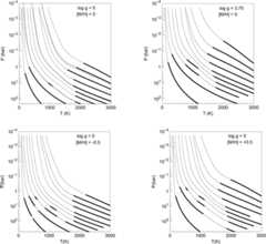
Figure 1. Converged radiative-convective equilibrium temperature profiles computedby our modeling approach for various parameters as noted in each panel.In all panels, models are shown every 200 K fromTeff = 200 to 1200 K and then every 300–2400 K. Thick linesshow convective regions of the atmospheres. Note how at higher effectivetemperatures the boundary lies near 2000 K, then with fallingTeff, convection turns on in some portions of the radiativeregion, until finally these isolated zones merge and the boundary movesup to near 1 bar in the coolest models. Dashed curves show cloudless,chemical equilibrium profiles from Phillips et al. (2020) for andTeff = 600, 1200, and 2100 K.
Download figure:
Standard imageHigh-resolution image
For most cases the lowermost radiative-convective boundary falls around 2000 K atwhich temperature the peak of the Planck function falls near theH-band spectral window in water opacity, permittingcooling to space. As expected from stellar atmosphere theory, the higher overallopacity of higher metallicity models shifts the entire structure to lowerpressures for the same effective temperature and gravity.
2.3. Opacities
We consider the opacity of 20 molecules and five atoms (see Table2). Details on how line widths areapplied to a given line list and the opacity calculation in general arepresented in Freedman et al. (2008,2014) andLupu et al. (2014). Sincethose publications we have updated several notable sources of opacity includingH2O, CH4, the alkali metals, and FeH. Below we discussour opacity sources for these species as well as our construction of opacitytables for use in the radiative-convective model and for the calculation ofhigh-spectral-resolution spectra. We note that opacity line lists are constantlybeing updated and it is necessary to freeze the choice of line lists in order toproduce a model set. Future versions of the Sonora models will include updatedopacities as warranted.
Table 2. Molecular Opacity Sources
| Molecule | Opacity Source(s)a | Line Widthsb |
|---|---|---|
| C2H2 | H12 | W16 |
| C2H4 | H12 | air |
| C2H6 | H12 | air |
| CH4 | Yurchenko et al. (2013),Yurchenko & Tennyson (2014)d;13CH4 STDS | P92 |
| CO | HT10; isotopologues Li etal. (2015) | L15 |
| CO2 | Huang et al. (2014) | scale |
| CrH | Burrows et al. (2002) | lin. |
| FeH | Dulick et al. (2003);Hargreaves et al. (2010) | lin. |
| H2O | Tennyson & Yurchenko(2018);isotopologues (HDO not included) Barber et al. (2006) | UCL |
| H2S | ExoMold; Azzam et al. (2015); isotopologues H12 | K02 |
| HCN | Harris et al. (2006); Harris etal. (2008);isotopologues GEISAf | lin. |
| LiCl | Weck et al. (2004)c | lin. |
| MgH | Weck et al. (2003)c | lin. |
| N2 | H12 | air |
| NH3 | Yurchenko et al. (2011) | W16 |
| OCS | H12 | W16 |
| PH3 | Sousa-Silva et al. (2015)d | S04 |
| SiO | Barton et al. (2013); Kurucz(2011)f | lin. |
| TiO | Schwenke (1998); Allardet al. (2000) | lin. |
| VO | McKemmish et al. (2016);ExoMol | lin. |
Notes.
aH12 = HITRAN 2012 (Rothman et al.2013);http://www.cfa.harvard.edu/hitran/updates.html; HT10= HITEMP 2010 (Rothman et al.2010);http://www.cfa.harvard.edu/hitran/HITEMP.html . blin. = linear estimate forγ, see text;air = air widths from H12; scale = 1.85 × self broadening; K02 =Kissel et al. (2002); L15 = Li et al. (2015); P92 = Pine (1992); S04 = Salemet al. (2004);W16 = Wilzewski et al. (2016); UCL = ExoMol web paged. chttp://www.physast.uga.edu/ugamop/. dhttp://www.exomol.com (Tennyson& Yurchenko2012). ehttp://ether.ipsl.jussieu.fr/etherTypo/?id=950. fhttp://kurucz.harvard.edu/molecules.html.Download table as: ASCIITypeset image
2.3.1. Neutral Alkali Metals and Atoms
We use a new calculation of atomic line absorption from the neutral alkalimetals (Li, Na, K, Rb, and Cs). These are now included using the VALD3 linelist13 (Ryabchikova et al.2015). Atomic line profiles, with the exception of the Na I andK I D lines, are assumed to be Voigt profiles without applying a line cutoffin strength or frequency. The line width is calculated from the Van derWaals broadening theory for collisions with H2 molecules usingthe coefficient tabulated in the VALD3 database when available or from thecodes of P. Barklem (https://github.com/barklem) otherwise. In all cases theclassical Unsöld width (e.g., Kurucz & Avrett1981) is corrected for a background gas ofH2 and He rather than atomic H, accounting for thedifferences in polarization and reduced mass. The choice of line cutoff forthe atomic species, with the exception of the D lines, has no materialeffect on the models.
The D resonance doublets of Nai (∼0.59μm) and Ki (∼0.77μm)can become extremely strong in brown dwarf spectra and their line profilescan be detected as far as ∼ 3000 cm−1 from the line center in Tdwarfs (Liebert et al.2000; Burrows et al.2000a; Marley et al.2002). Under these circumstances, a Lorentzian line profilebecomes grossly inadequate in the line wings and a detailed calculation isrequired.
For these two doublets, we have implemented line-wing profiles based on theunified line-shape theory (Rossi & Pascale1985; Allard et al.2007a,2007b). The tabulated profiles (N. Allard2000, private communication) are calculated for the D1 and D2 lines of Nai and Ki broadened by collisions with H2and He, for temperatures ranging between 500 and 3000 K and at a referenceperturber (H2 or He) number density ofnpert = 1019 (K–H2 profiles) or1020 cm−3 (Na–H2, Na–He and K–Heprofiles). Two collisional geometries are considered for broadening byH2 and averaged to obtain the final profile. The line core isdescribed with a symmetric Lorentz profile with a width calculated from thesame theory, with coefficients given in Allard et al. (2007b).
The line profiles are provided as a set of coefficients in a densityexpansion that allows their evaluation at a range of densities other thanthe reference density of the tabulation. The third-order expansion isconsidered suitable up to perturber densities of 1020cm−3 (N. Allard, private communication) and the Lorentzianline width is linear in perturber density (Allard et al.2016). Using thoseexpressions and by interpolating in temperature, we produce a set ofprofiles covering 500–3000 K and on a uniform grid. In atmosphere models and spectra thatmay exceed these limits, we refrain from extrapolating. This is generallyacceptable since the Nai and Ki resonance doublets playa lesser role in the total opacity outside of these boundaries. Nonetheless,calculations that reach higher densities are valuable. After the modelspresented here were computed, Allard and collaborators presented new tablesfor K–H2 (Allard et al.2016) and Na–H2 (Allard et al.2019) valid to higher pressure. We will usethose tables in future updates to the model grid. Tests show that while thenew treatment does impact the model spectral slope near 1μm, it does not appreciably alter the temperatureprofiles from the present model generation.
2.3.2. FeH
For FeH we use the line list of Dulick et al. (2003) which was our opacity source inprevious models. However, this list did not include the E-A band at 1.6μm which is prominent in M and L dwarfs.Here we include this rovibrationalE4Πi −A4Πi electronic transition, employing a line list from Hargreaves et al.(2010). This list wasconstructed by fitting to empirical spectra of cool M dwarfs and tolaboratory measurements. As a consequence there are multiple uncertaintiesin the line list, including the lower energy level of many of the lines,which are set to a constant value. Hargreaves et al. (2010) ultimately applied an enhancementfactor of 2.5 to their initial line strengths in stellar-atmosphere modelsin order to match observations. In our own initial test models employingthis line list we found that the predicted band strength as seen in ourmodels was far in excess of that observed in early L dwarfs. Afterdiscussions with R. J. Hargreaves (2015, private communication) on varioussources of uncertainty we decided to reduce the line strengths for this bandonly by a factor of 1/3, slightly overcorrecting to remove the correctionfactor of 2.5 to better match observations. This is the only absorption bandin our entire model set for which we have applied such an empiricalcorrection.
2.3.3. Line Profiles
The proper choice of line widths to apply to each individual molecular lineis a difficult problem as there is often little to no theoretical orlaboratory guidance, particularly for higher quantum number transitions thatare important at higher temperatures. For each molecule we have applied thebest information available at the time our opacity database was constructedalthough in many cases we have had to estimate the broadening with limitedinformation. Table2summarizes our choices for line widths, including cases in which we usedliterature values or widths appropriate to air, rather than H2 −He mixtures.
In most molecular line lists, the maximumJquantum number is above 100. However, Lorentz broadening coefficients aretypically only available up toJ ∼ 50, whichwe termJlow. In such cases where data are lacking, we extrapolate thebroadening parameterγ by assuming a value, ∼0.075 cm−1 atm−1, for the lowestJ value in any set then adjusting the broadening at anyJ by a linear expression inJ −Jlow up to some maximumJ. AbovethatJ,γ isheld fixed at ∼ 0.04 cm−1 atm−1. A similar approachhas been followed by the UCL group (J. Tennyson 2018, privatecommunication).
2.3.4. Opacity Tables
Opacities are computed at each of 1060 distinct pressure-temperature pointscovering the range 75 ≤T ≤ 4000 K and10−6 ≤P ≤ 300 bar on awavenumber grid constructed such that there are about 3 points per Dopplerwidth for the H2O molecule. This typically amounts to roughly 2 ×10⁶ individual points for intermediateT andP with up to107 points at the lowest pressures at which we compute theopacity from up to 1010 individual spectral lines (for example,in the case of CH4). This tabulated opacity is used both inpost-processing to construct high-resolution spectra for individual modelsand also to computekcoefficients which areused to calculate the atmospheric structure.
To calculate thekcoefficient we sum thecontribution of every molecule to the total molecular opacity by weightingby their relative equilibrium abundances (see next section). Within each of190 spectral bins covering the wavelength range 0.4 to 320μm, we then compute thekcoefficients using the summed opacity. We note that this is moreaccurate than later combiningkcoefficientscomputed for individual gases (e.g., Lacis & Oinas1991; Amundsen et al.2017). This approach, however, removesflexibility in adjusting local gaseous mixing ratios, for example, toaccount for disequilibrium chemistry effects (see Amundsen et al.2017 for a recentdiscussion). We use 8 Gauss points for thekcoefficients, following a double Gaussian scheme in which 4 pointscover the range 0 to 0.95 of the cumulative distribution and 4 additionalpoints cover the range 0.95 to 1.00. This permits more precise resolution ofthe strongest few percent of the molecular lines within any given spectralbin. Tests (M. Line 2020, private communciation) have shown that thisdouble-Gauss approach yields essentially identical thermal profiles as thosecomputed with 20 Gauss points covering the full distribution range of 0 to1.0 and the same opacities. Thekcoefficientsfor all of the model cases presented here are available for downloadhere.
In addition to these opacity sources we also account for several othercontinuum opacity sources. Pressure-induced opacity fromH2–H2, H2–H, H2–He,H2–N2, and H2–CH4 isaccounted for as described in Saumon et al. (2012). We also include bound–free andfree–free opacity from H− and and free–free opacity from
 and He− as well as electron scattering.Rayleigh scattering from H2, H, and He is also included. We notein passing that, despite the recent “discovery” of the importance ofH− opacity in transiting planet atmospheres14, H− has long been recognized as an important source ofcontinuum opacity in cool stars (Chandrasekhar & Münch1946). Our models havealways included this opacity source since Marley et al. (1996). The models in thispaper do not include cloud opacity; our method for accounting for suchopacity will be presented in a future paper in the series.
2.4. Radiative Transfer
In the radiative-convective model we compute radiative fluxes through each modellayer using the “two-stream source function method” outlined in Toon et al.(1989). This scheme firstcomputes a two-stream (up and down) solution to the flux and then uses thetwo-stream solution as the source function for scattering in the secondcalculation step that computes the flux in six discrete beams. Following Toon etal., within each model layern, with optical depthranging fromτ = 0 at the top toτ =τbot at the bottom, the source function is linearized asBn(τ) =B0n +B1nτ whereB0n is the Planck function at the temperature at the top of the layer andB1n = [B(T(τbot)) +B0n]/τn. The final upward and downward fluxes are computed by integration overthe multiple streams. The method is exact for pure absorption and provides anacceptable balance between accuracy and speed for cases with particlescattering. Toon et al. (1989) provide tables of the size of the error in various cases. Thelower and upper boundary conditions are those commonly used in the stellaratmospheres problem for semi-infinite atmospheres (Hubeny & Mihalas2014). Recently, Heng &Kitzmann (2017) have extendedthe Toon et al. method for greater accuracy in strongly scattering atmospheres,a limit we do not reach in the cloudless models presented here.
Once we have a convergedT(P) model we compute high-resolution spectra by solving theradiative transfer equation for nearly 362,000 monochromatic frequency pointsbetween 0.4 and 50μ m. The monochromaticopacities are calculated from the same opacity database, line broadening, andchemistry tables as thekcoefficients and arepre-tabulated on the same (T,P) grid. In these cloudless models, the radiative transferequation is solved with the Rybicky solution (Hubeny & Mihalas2014) assuming that Rayleighscattering is isotropic. The resulting spectral energy distributions are inexcellent agreement with those obtained from the lower-resolutionk-coefficient method with their respective integratedfluxes differing by less than 2% in nearly all cases.
2.5. Chemical Equilibrium
Chemical equilibrium abundances at the grid (P,T) points were calculated using a modifiedversion of the NASA CEA Gibbs minimization code (see Gordon & McBride1994) based upon priorthermochemical models of substellar atmospheres (Fegley & Lodders1994,1996; Lodders1999,2002; Lodders & Fegley2002; Visscher et al.2006,2010; Visscher2012) and recently used to explore gas andcondensate chemistry over a range of atmospheric conditions (Morley et al.2012,2013; Moses et al.2013; Kataria et al.2016; Skemer et al.2016; Burningham et al.2017; Wakeford et al.2017).
Equilibrium abundances (with a focus on key constituents that are included in theopacity calculations: H2, H, H+, H−, , He, H2O, CH4, CO, CO2, OCS,HCN, C2H2, C2H4,C2H6, NH3, N2, PH3,H2S, SiO, TiO, VO, Fe, FeH, MgH, CrH, Na, K, Rb, Cs, Li, LiOH,LiH, LiCl, and e−) were calculated over a wide range of atmosphericpressures (1μbar to 300 bar) and temperatures (75to 4000 K) and over a range of metallicities (−1.0 dex to +2.0 dex relative tosolar abundances, assuming uniform heavy-element enrichment), and C/O elementabundance ratios (0.25 to 2.5 times the solar C/O abundance ratio of C/O =0.458) using protosolar abundances from Lodders (2010) which represent the bulk solar systemcomposition and provide continuity with earlier iterations of the chemicalmodels. Other C/O ratios can be adopted (e.g., 1.25 × C/O, corresponding to C/O= 0.57) for consistency with more recent determinations of the photospheric C/Oratio (e.g., Asplund et al.2009; Caffau et al.2011; Lodders2020; Asplund et al.2021).
For a given metallicity, variations in the C/O ratio were computed while holdingthe C+O abundance constant, so that the total heavy-element abundance relativeto hydrogen (Z/X),characterized by [M/H], remains constant. For example, to achieve C/O ratiosgreater than the solar value (e.g., 1.25 × or 1.5 × the adopted solar ratio ofC/O = 0.458), the oxygen abundance is slightly diminished while the carbonabundance is slightly enhanced. For most species, we utilized the thermochemicaldata of Chase (1998) withadditional thermochemical data from Gurvich et al. (1989,1991,1994),Burcat & Ruscic (2005),and Robie & Hemingway (1995) for several mineral phases.
Condensation from the gas phase is included with the “rainout” approach ofLodders & Fegley, wherein condensates are removed from the gas mixture lyingabove the condensation level. This prevents further gas-condensate chemicalreactions from occurring higher up in the atmosphere, above the condensationpoint. Rainout has been validated for alkali species by the sequence of thedisappearance of Na and K spectral features (Marley et al.2002; Line et al.2017; Zalesky et al.2019).
As in previous thermochemical models, the equilibrium abundance of anycondensate-forming species at higher altitudes is determined by its vaporpressure above the condensate cloud (Visscher et al.2010). The detailed equilibria models ofLodders (2002) show thatseveral elements (such as Ca, Al, Ti) may be distributed over a number ofdifferent condensed phases depending upon pressure and temperature conditions.For simplicity, here we consider the vapor pressure behavior of TiO and VO inequilibrium with Ti2O3, Ti3O5, orTi4O7, and V2O3,V2O4, and V2O5, respectively, aswe are primarily interested in the behavior of Ti and V above the cloud deck andthe current grid lacks the resolution for detailed Ca–Ti equilibria as afunction of temperature. The behavior of Mg-, Si-, and Fe-bearing gases wascalculated following the approach of Visscher et al. (2010) and included the equilibrium condensationof forsterite (Mg2SiO4), enstatite (MgSiO3),and Fe metal. As in Lodders (1999), major condensates for the alkali elements included LiCl, LiF,Na2S (see also Visscher et al.2006), KCl (see also Morley et al.2012) RbCl, and CsCl.
2.6. Comparison to Other Approaches
As mentioned above, the construction of any forward model involves numerouschoices and trade-offs. When comparing models from different groups, it is worthkeeping in mind the various approximations and assumptions behind the models.Here we highlight a few such differences.
Our modeling scheme, with roots in solar system atmospheres, was first applied toa brown dwarf (Gl 229 B) in Marley et al. (1996). That same year, Allard et al. (1996) likewise applied thePHOENIX modeling scheme, with roots in stellaratmospheres, to the same object. Both models developed over time with thePHOENIX model ultimately producing the widely citedCOND andDUSTY model sets(Allard et al.2001). Incontrast to our approach of using pre-tabulated chemistry and opacities, thePHOENIX model computes chemistry and opacities on thefly.COND also employs full equilibrium chemistry ratherthan rainout chemistry to compute molecular abundances. As we note above, recentretrieval studies have validated rainout chemistry in the context of T dwarfs.To compute fluxes,PHOENIX uses the sampling method inwhich the radiative transfer is only computed at a finite number (∼105 or more, T. Barman 2017, private communication) ofwavelength points. Our method accounts for the opacity and uses the informationat many more (106–107) points, but only in a statisticalsense as the opacity distribution within wavelength bins is described bykcoefficients.
A more recent version of thePHOENIX model is known asBT-Settl (Allard et al.2014),where the BT denotes the source of the water opacity employed (Barber et al.2006) and the Settldenotes the handling of condensate opacity. These models have not been asthoroughly described and a more detailed comparison is not yet possible.
Recent studies of radiative transfer for transiting planets have found that thek-coefficient method more closely reproducescalculations performed at very high spectral resolution that the samplingmethod, since the entire range of both low- and high-opacity wavelengths isconsidered (Garland & Irwin2019). In practice, for most of the atmospheres considered here,this is unlikely to be a major difference. However, our own tests of fluxescomputed with opacity sampling find that at low temperatures, where there arerelatively few opacity sources and the opacity can vary wildly with wavelength,sampling can produce large errors unless many more points are employed thantypically used. A systematic comparison between the approaches would beinformative. Differences between the approaches in the context of cloud opacitywill be discussed in a future paper.
Another widely cited model set is that of the Adam Burrows’s group which consistsof two different approaches. The models presented in Burrows et al. (1997,2001) were computed using the Marley et al.(1996,1999) radiative-convectivemodel described above. After 2001 the Burrows group transitioned to a modelingframework based on a widely used stellar atmospheres codeTLUSTY (Hubeny1988; Hubeny & Lanz1995) adapted for use in brown dwarfs (e.g.,Burrows et al.2002,2004,2006). This work uses the sampling method tohandle opacities, likePHOENIX, but with the ability tohandle rainout and quenching (Hubeny & Burrows2007) rather than relying on pure equilibriumchemistry. There are also differences in the treatment of radiative transfer andthe global numerical method used to solve the set of structural equations.Hubeny (2017) provides athorough, critical comparison of various approaches employed in substellarmodels.
Recently Malik et al. (2017)released the open-source atmosphere radiative-equilibrium modeling frameworkHELIOS. As of this date the model structures arestrictly in radiative equilibrium.HELIOS computesatmospheric structure assuming true chemical equilibrium, not rainout chemistry,using a fast analytic approximation of the C, N, O chemistry (Heng et al.2016). The model useskcoefficients of individual molecules which theycombine on the fly using “random overlap” approximation rather than thepre-mixed opacity tables employed here or the “re-bin and re-sort” methodusually used to combinekcoefficients (seeAmundsen et al.2017). Whilefast, this approximation can produce large flux errors in certain cases because,in fact, the opacities are not random but are vertically correlated through theatmosphere (Amundsen et al.2017). There has not yet been a systematic comparison of modelatmospheres computed byHELIOS with other models usingmore traditional methods for computing non-irradiated substellaratmospheres.
As noted in Section1, the modelset most similar to our own is Phillips et al. (2020). Those authors made generally similarmodeling choices, including rainout equilibrium, although for the opacities,they mix single-gask coefficients followingAmundsen et al. (2017) ratherthan pre-computing them for the mixture, as we do here. They do not discusswhether their models produce multiple layer convection zones, although itappears from their posted structures that they in fact do, with generallysimilar structure as our Figure4.Their models are only for solar metallicity and those authors advise users toonly trust models belowTeff = 2000 K, despite the grid going to higher temperatures as theyneglect some important opacity sources. Where they can be compared, the PhillipsT(P) profilesare very similar to our own, as seen in Figure1, except above 2000 K where they are slightlycooler, as expected given their neglect of some opacities.
When comparing atmospheric abundances computed by our approach and other methodsit is crucial to consider the impact of our rainout chemistry assumption (see,e.g., Lodders & Fegley2006). Because of rainout, certain species that can potentially besignificant sinks of atoms of interest, do not form. For example, under rainoutconditions, Fe2O3, does not form as the Fe condensate isremoved from the atmosphere. Rainout atmospheres cooler than the iron oxidecondensation temperature will thus appear to have larger O abundances than othertreatments with the same initial O abundance. Likewise, rainout causes theremoval of condensed aluminum oxide Al2O3 from theatmosphere, preventing the formation of albite (NaAlSi3O8)which would otherwise remove atomic sodium from the atmosphere at about 1000 K.Retrieval studies have shown (Zalesky et al.2019) that the rainout chemistry prediction ismost consistent with the observed spectra of T dwarfs.
The rainout chemical equilibrium abundance tables used to compute the modelspresented here are available along with the models at our model page.15
2.7. Evolution Model
The model for the interior and the evolution is discussed in detail in Saumon& Marley (2008;hereafter,SM08). Briefly,the interior is modeled as fully convective and adiabatic and uses theatmosphere models described herein as the surface boundary condition. Wegenerate sequences for the three metallicities of the atmosphere models ([M/H] =−0.5, 0 and 0.5). The models are started with a large initial entropy (“hotstart”) and include fusion of the initial deuterium content.
We incorporate three significant improvements over the models ofSM08. First, we now account formetals in the equation of state by using an effective helium mass fraction(Chabrier & Baraffe1997)

whereY = 0.2735 is the primordialHe mass fraction andZ the mass fraction of metals(Z = 0.00484, 0.0153 and 0.0484, correspondingto [M/H] = − 0.5, 0,and +0.5, respectively). The hydrogen and helium equations of state are from thetables of Saumon et al. (1995), as inSM08.Second, we use the improved nuclear-reaction screening factors of Potekhin &Chabrier (2012). Third, thenew surface boundary condition is provided by the atmospheres presented herewhich are defined over a finer (Teff, ) mesh and extend to lower gravity (
 ) and lowerTeff = 200 K. This allows modeling of lower mass objects, down to 0.5MJ.
2.8. Previous Applications
Our group has applied the same basic modeling approach described here to a numberof topics related to ultracool dwarfs and extrasolar giant planets. This work isgenerally summarized in Marley & Robinson (2015). Notable applications have includedcomputation of the evolution tracks presented in Burrows et al. (1997), characterization of L andT dwarfs from their near-infrared spectra in Cushing et al. (2008) and Stephens et al. (2009), calculation ofatmospheric thermal profiles of irradiated giant planets (Fortney et al.2005), and modeling of youngdirectly imaged planets in (Marley et al.2012). Our prediction that the clearing ofclouds at the L/T transition would result in an excess of transition browndwarfs (Saumon & Marley2008) was recently validated with the 20 pc brown dwarf census ofKirkpatrick et al. (2021).
In addition, Fortney et al. (2008) investigated the atmospheric structure and spectra ofcloud-free gas giants from 1–10 Jupiter masses, for models withTeff < 1400 K. The role of enhanced atmospheric metallicity, anoutcome expected from the core-accretion model of planet formation (e.g.,Fortney et al.2013), wasinvestigated as a way to observationally distinguish planets fromstellar-composition brown dwarfs. These atmosphere models were coupled to the“cold start” and “hot start” evolutionary tracks of Marley et al. (2007) to better understand themagnitudes and detectability of young giant planets. Later, Fortney et al.(2011) modeled theevolution of the atmospheres of the solar system's giant planets to investigatehow metal enrichment and the time-varying (but modest) insolation effect ourunderstanding of the cooling history of these planets.
While earlier models included the iron and silicate clouds that form in L-dwarfatmospheres, Morley et al. (2012) considered the salt and sulfide clouds (Visscher et al.2006) that likely form incooler T-dwarf atmospheres, finding that models that included the formation ofthese additional species could better match the colors of the T-dwarfpopulation. Morley et al. (2014b) focused on even colder objects, the Y dwarfs, many of whichare cold enough to condense volatiles like water into ice clouds. Morley et al.(2014a) considered howeither clouds or hot spots could cause wavelength-dependent variability in T-and Y-dwarf spectra.
3. Model Results
3.1. Thermal and Composition Profiles
Radiative-convective equilibrium thermal profiles are shown for a selection ofmodel parameters in Figure1 fortwo gravities at solar metallicity and two metallicities at fixed gravity. Thegeneral behavior of the extent of the convection zones apparent in previous workis also seen here. At the highest effective temperatures the singleradiative-convective boundary lies near 2000 K and at pressures in the range of1–0.01 bar, depending on gravity. As the effective temperature falls the top ofthis convection zone stays near 2000 K but moves to progressively higherpressures. Finally, for effective temperatures below 1000K, the denser regionsof the atmosphere begin to be cooler than about 1000 K, resulting in the peak ofthe local Planck function lying not in the relatively clear, low-opacity regionsfrom 1 to 2μm but rather in the higher gasopacity region between 2 and 4μm. Consequently, asecond detached convection zone forms around 1000 K.
The second transition from convective to radiative transport occurs whensufficient flux can emerge through the spectral window at 4 to 5μm. In some cases a third, small convection zonebriefly develops higher in the atmosphere. Finally, with falling effectivetemperature, these detached zones merge and the atmosphere is finally fully, oralmost fully, convective all the way up to about 0.1 to 1 bar, depending ongravity. The universality of ∼ 0.1 bar radiative-convective boundaries at lowTeff andg has been explored by Robinson& Catling (2014).
Correctly mapping the detached convection zones is important for the evolutioncalculation as they change the atmospheric temperature gradient away from thatof pure radiative equilibrium. This in turn alters the temperature andpressure–and thus atmospheric entropy–of the deep radiative-convective boundary,which ultimately controls the thermal evolution of the entire object.
Likewise, this behavior of the radiative regions rapidly merging, raising theradiative-convective boundary to pressures near 1 bar at cooler effectivetemperatures is likely the explanation for the rapid rise in the eddy-mixingcoefficient, as inferred from observed disequilibrium chemistry below 400 K(Miles et al.2020).
3.2. Model Spectra
All of the model spectra described in this paper are available online.16 Here we briefly describe the characteristics of the model set.
Spectra for a selection of model cases and wavelength ranges are shown in Figures2 through7. While these cloudless models are of course lessrelevant to observed spectra through much of the L-dwarf regime, they arenevertheless instructive for illustrating how the atmospheric chemistry evolvesas effective temperature falls through the M, L, T, and Y spectral types.
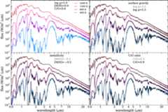
Figure 2. Overview of complete model spectra for various combinations of surfacegravity, metallicity, and C/O ratio. The line color labels the effectivetemperature as shown in the upper left panel. Spectral resolutionR varies across the figure forclarity. Effective temperatures are as labeled in the top left panel.Models shown in the top left panel are repeated in the other threepanels along with two variations (in gravity, metallicity, and C/Oratio) in black and gray, as labeled in each sub-panel. Of particularinterest is the effect of metallicity onK-band emission (Fortney et al.2008).
Download figure:
Standard imageHigh-resolution image
As the atmosphere cools, molecular features become more prominent and the roughlyblackbody spectra apparent at 2400 K is nearly unrecognizable by 400 K (Figure2). The universality of theM-band flux excess, first noted in Marley etal. (1996), is apparent asare the familiar excesses inY,J,H, andK bands. All of these arise from opacity windowsallowing flux to escape from deep-seated regions of the atmospheres where thelocal temperature often exceedsTeff. The folly, for most purposes, of attempting to describe thethermal emission of brown dwarfs or self-luminous planets as beingblackbody-like is evident from casual inspection of Figure2.
Spectral sequences for limited spectral ranges are shown in Figures3 through7. The red optical (Figure3) is primarily sculpted by the K I resonancedoublet centered around 0.77μm (Burrows et al.2000b). Because thisspectral region otherwise has low gas opacity, the influence of the K absorptionlingers in these cloudless models well below theTeff at which potassium condensates form (around 700 K). Including theeffects of the Na and K condensates changes the opacity as shown by Morley etal. (2012), but in thepresent cloudless models deep-seated K still influences the spectra down toTeff ∼ 400 K. Finally, at the lowest effective temperatures, thesignatures of water and methane appear, strikingly altering the predictedoptical spectra redward of 0.80μm.
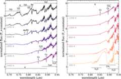
Figure 3. Red optical spectral sequence (R ∼ 2000) ofmodels for solar metallicity and C/O ratio at , shifted vertically for clarity. Notable absorptionfeatures are labeled.
Download figure:
Standard imageHigh-resolution image
Figure4 depicts the crucialnear-infrared region. With fallingTeff the familiar gradual departure of the refratory species and thealkalis, as well as the appearance of methane are apparent. The cloudless modelsare cooler than models that account for condensate opacity, thus methane appearsaroundTeff = 1600 K inH band, which is warmerthan it is seen in nature (Kirkpatrick2005). The progressive loss of flux in theK band, attributable to the increasinginfluence of pressure-induced opacity of molecular hydrogen, continues throughthe entire sequence. The flux peaks are progressively squeezed between strongerand stronger molecular absorption until, by 300 K, they become sharp and wellseparated. As in the previous figure, the coldest model shown, at 300 K, has anotably different morphology as ammonia features are apparent near 1μm. This interesting small spectral region is furtherexpanded in Figure5.
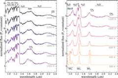
Figure 4. Same as Figure3, but forfar-red through near-IR spectral range withR ∼ 600.
Download figure:
Standard imageHigh-resolution image
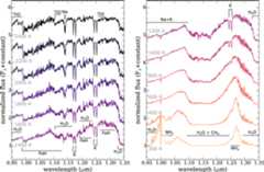
Figure 5. Same as Figure3, buthighlighting the spectral region near 1μmwithR ∼ 1500. In the coldest models, theloss of almost all major gaseous absorbers, particularly the alkalimetals, except H2O, NH3, and CH4,transforms the appearance of this spectral region.
Download figure:
Standard imageHigh-resolution image
The wavelength range to be explored in fresh detail by the James Webb SpaceTelescope beyond 3μm is explored in Figures6 and7. This is a region broadly sculpted by wateropacity with important contributions from methane and ammonia at lower effectivetemperature. The 5μm spectral window allowsdeep-seated flux to emerge, as in familiar images of Jupiter (e.g., Orton et al.1996). The long pathlengths through the atmosphere, as in the near-infrared, permit detection ofrare molecules (Morley et al.2019). Gharib-Nezhad et al. (2021) consider the detectability oflithium-bearing molecules in this region.
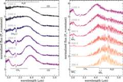
Figure 6. Same as Figure3, but forthe 3 to 5μm spectral region andR ∼ 1000. Note how the peak in emission shiftsfrom ∼4 to ∼ 4.5μm through thissequence.
Download figure:
Standard imageHigh-resolution image
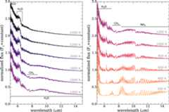
Figure 7. Same as Figure3, but forthe mid-IR spectral range withR ∼ 1000.Note how the arrival of NH3 dramatically transforms thisregion below about 1200 K in these equilibrium chemistry models.
Download figure:
Standard imageHigh-resolution image
Figure8 explores the influence ofthe C/O ratio in the near-infrared among the coolest models where differences inmethane abundance are most notable. Although these are pure chemical equilibriummodels, the influence of disequilibrium chemistry is less notable in thisspectral region at these cool effective temperatures, thus providing bettertracers of the atmospheric C/O ratio, with the usual caveat of accounting forloss of O into condensates at higher temperatures.
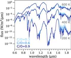
Figure 8. Comparison of model spectra (R ∼ 300) for at threeTeff and three C/O ratios as indicated. Note that the 400 and200 K models have been scaled down by 102 and 104,respectively, for clarity in plotting. Note that the indicated C/Oratios are for the bulk gas composition and not the gas composition inthe photosphere probed here, as about 20% of the O atoms are lost tosilicate-grain formation deeper in the atmosphere.
Download figure:
Standard imageHigh-resolution image
Finally9 compares the modelspectra presented here to our earlier generation of models (Saumon et al.2012) through the effectivetemperature range of the T and Y dwarfs. The most notable differences arise fromchanges in the alkali D line treatment and updated ammonia and methane opacity(Section2.3). We have foundthat more recent updates to the molecular line lists generally are not similarlyapparent at the illustrated spectral resolutionR∼ 1000, but do appear at much higher spectral resolutionR > 10,000.
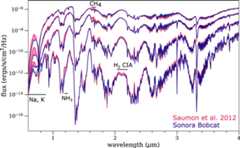
Figure 9. Comparison of the present Sonora Bobcat model spectra (R ∼ 1000) with those of Saumon et al. (2012) atTeff = 1300, 900, 500, and 300 K (top to bottom). Absorbersresponsible for notable differences are labeled.
Download figure:
Standard imageHigh-resolution image
3.3. Evolution
The newly computed evolution tracks are shown in Figures10 and11. The extension of the surface boundary condition to lowerTeff illuminates an interesting feature of Y-dwarf evolution. TheSM08 models were based onatmospheres that extended only to 500 K and the corresponding boundary conditionwas extended to lowerTeff with a plausible, constrained extrapolation. That extrapolationwas inaccurate because it did not account for the condensation of water, whichthe new low temperature atmosphere models include. As water is the dominantabsorber in lowTeff Y dwarfs, its disappearance belowTeff < 400 K results in more transparent atmospheres, which affectsthe evolution.

Figure 10. Low-temperature end of the cooling tracks of brown dwarfs inTeff and gravity for the sequence based on cloudlessatmospheres of solar metallicity. The evolution proceeds from right toleft along the heavy black lines, which are labeled with the mass inM⊙ (the unlabeled track at the bottom hasM = 0.001M⊙). Light gray cooling tracks are from Saumon & Marley(2008).Isochrones are shown by the blue dotted lines: (from right to left)0.01, 0.02, 0.04, 0.1, 0.2, 0.4, 1, 2, 4, and 10 Gyr. The nearlyvertical red lines are curves of constant luminosity: (from left toright): , to −5 in steps of 0.5. Curves of constant radius areshown in green: (from top to bottom) 0.08 to 0.13R⊙ in steps of 0.01. The phase of deuterium burning isrevealed by the kink in the isochrones for objects with masses between0.01 and 0.015M⊙.
Download figure:
Standard imageHigh-resolution image

Figure 11. Late evolution of the luminosity of low-mass ultracool dwarfs. Thepresent Sonora models (solid lines), include water condensation andremain more luminous (cool more slowly) belowTeff ∼ 400 K than the Saumon & Marley (2008) models (SM08, dotted lines).Each curve is labeled by the mass. The more massive dwarfs are notaffected as they remain hotter than 400 K over the age of the Galaxy(see Figure10).
Download figure:
Standard imageHigh-resolution image
The impact of this accounting for water condensation can be seen in Figure10 as a divergence in therespective cooling tracks of low-mass objects ( < 0.01M⊙) belowTeff ∼ 400 K. The new models have slightly higher gravity andluminosity (Figure11).Qualitatively, this is similar to the hybrid model ofSM08 for the L/T transition where thedisappearance of cloud opacity causes a pileup of brown dwarfs at the transition(Kirkpatrick et al.2021),although the effect appears to be weaker.
This result should not be taken at face value, however. The present cloudlessmodel atmospheres include condensation of water but not the resulting cloudopacity. Unlike magnesium-silicate clouds, which have considerable opacity butwhose gas phase precursors (e.g., MgH) have barely been detected in spectra(see, e.g., Kirkpatrick2005)and thus have negligible opacity, water is the dominant gas-phase absorberthroughout the L-T-Y sequence. Thus, water condensation transforms the opacityfrom a series of strong molecular bands throughout the near- and mid-IR to acontinuum of condensate opacity. Until Y-dwarf models with a reliabledescription of water clouds are produced, the net effect of water condensationon very cool brown dwarf evolution will remain uncertain.
The effect of metallicity on the coolings tracks is shown in Figure12 for the luminosity and Figure13 forTeff. Generally, the higher-metallicity models are slightly moreluminous at a given age because the higher opacity of the atmosphere slows theircooling. All masses show the same trend with![${\rm{\Delta }}\mathrm{log}L/{\rm{\Delta }}[{\rm{M}}/{\rm{H}}]\lesssim 0.15$](/image.pl?url=https%3a%2f%2fcontent.cld.iop.org%2fjournals%2f0004-637X%2f920%2f2%2f85%2frevision2%2fapjac141dieqn15.gif&f=jpg&w=240) . Deuterium burning causes the apparent anomalies in the 0.01and 0.02M⊙ tracks. The 0.07M⊙ tracks are just below the hydrogen-burning minimum mass (HBMM).Since the HBMM decreases with increasing metallicity, the [M/H] = +0.5 modelapproaches a main-sequence equilibrium state while the others do not produceenough nuclear energy to prevent further cooling. The evolution ofTeff is very similar to that ofLbol.
. Deuterium burning causes the apparent anomalies in the 0.01and 0.02M⊙ tracks. The 0.07M⊙ tracks are just below the hydrogen-burning minimum mass (HBMM).Since the HBMM decreases with increasing metallicity, the [M/H] = +0.5 modelapproaches a main-sequence equilibrium state while the others do not produceenough nuclear energy to prevent further cooling. The evolution ofTeff is very similar to that ofLbol.

Figure 12. Comparison of brown dwarf luminosity cooling tracks for three differentmetallicities. Each triplet of tracks is labeled with the mass in solarmasses. For a given mass and age, a higher metallicity results in aslightly higher luminosity. The 0.07M⊙ models are just below the hydrogen-burning minimum mass andtheir fates diverge after 2 Gyr, depending on the metallicity. The [M/H]= +0.5 track approaches a stable equilibrium on the main sequence whilethe lower metallicity tracks for that mass fail to do so.
Download figure:
Standard imageHigh-resolution image

Figure 13. Same as Figure12, but forthe effective temperature.
Download figure:
Standard imageHigh-resolution image
Because of the systematic differences that persist between forward model spectraand data, determinations ofTeff and especially the gravity, by fitting observed spectra remainrather uncertain. Atmospheric parameters determined from models from differentgroups often disagree (e.g., Patience et al.2012). However, the modeled bolometricluminosity, because it integrates over all wavelengths, is much less sensitiveto such model errors and can also be determined fairly reliably fromobservations. Benchmark brown dwarfs, either bound in a binary system with amore easily characterized primary star or members of a moving group also havewell determined metallicities and fairly well constrained ages. Equipped withLbol, [M/H] and the age, the mass (e.g. Figure12),Teff, radius, and gravity follow from evolution sequences with a gooddegree of confidence.
The evolution sequences are available for all three metallicities.17 The tables provide mass, age, radius, luminosity, gravity, andTeff along cooling tracks at constant mass and, for convenience, alongisochrones, along constant luminosity curves, and for a given pair of (Teff, ). The moment of inertiaI isalso provided for each mass as a function of time. For a spherically symmetricbody of radiusR,
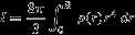
which is a useful quantity for studies of the angular momentum ofbrown dwarfs and their deformation under rotation (Barnes & Fortney2003; Sengupta & Marley2010; Jensen-Clem et al.2020).
4. Comparisons to Selected Data Sets
4.1. Spectra
Spectra from the Sonora Bobcat model set have already been used in a number ofcomparisons to various spectral data sets. The most systematic application hasbeen in Zhang et al. (2021a)and Zhang et al. (2021b) whoapplied the Bayesian inference tool Starfish to near-infrared spectra (R ∼ 80–250) of 55 late-T dwarfs, including threebenchmark (T7.5 and T8) objects. While good spectral fits could be found betweenmodel library and observed spectra, there were certain consistent discrepanciesacross most all objects. Most notably, the peak of theJ-band in the best-fit spectra was too bright for most objects,while the peak of theH band was too dim. In bothcases, the discrepancy increases with fallingTeff and later spectral types. Zhang et al. (2021b) attributed these discrepancies to deepclouds and disequilibrium chemistry, respectively, although further modeling isneeded to understand this in detail.
Zhang et al. (2021b) also usedthis model set to quantify the well known degeneracy between metallicity andgravity by considering all of the model spectra. They found that thegravity–metallicity degeneracy can be described with![${\rm{\Delta }}\mathrm{log}g\sim 3.42{\rm{\Delta }}[{\rm{M}}/{\rm{H}}]$](/image.pl?url=https%3a%2f%2fcontent.cld.iop.org%2fjournals%2f0004-637X%2f920%2f2%2f85%2frevision2%2fapjac141dieqn17.gif&f=jpg&w=240) . In other words, a change of +0.1 in [M/H] has nearly the sameeffect as a change in
. In other words, a change of +0.1 in [M/H] has nearly the sameeffect as a change in of about 0.34.
At higher spectral resolution, the models generally reproduce the finer spectralstructure of cloudless objects fairly well. Comparing among three model sets,for example, Tannock et al. (2021) found Sonora-Bobcat models had the lowestχ2 inJ,H, andKbands when compared toR ∼ 6000 spectra of a T7 dwarf; this is likely due toour choice of recent molecular opacity tables (Table2) and illustrates the value of considerable effortthat underlies the calculation of these tables.
4.2. Colors
The online tables contain model photometry in a selection of photometricpassbands, including the MKO, WISE, SDSS, 2MASS, Spitzer/IRAC, and JWST systems.Model absolute magnitudes are computed using radii from the evolution model.Figure14 shows our predictedSonora Bobcat model photometry on the familiar ultracool dwarfJ versusJ−K color–magnitude diagram along with a sample of fielddwarfs and subdwarfs selected from Best et al. (2020) for having well constrained photometry anddistances. Model colors are shown for three gravities and threemetallicities.

Figure 14. Sonora Bobcat cloudless colors for different constant values of gravityand metallicity as compared to Maunakea ObservatoryJ- andK-band photometry ofnearby M, L, T, and Y dwarfs from Best et al. (2020). The curves are coded by theirline types (solid, dashed, dotted) for , 4, and 3, respectively, and line colors, from top tobottom groups [M/H] = − 0.5, 0.0, and +0.5 for red, black, and green.The near-infrared spectral types are denoted by the color of the dot.Half-filled circles are subdwarfs.
Download figure:
Standard imageHigh-resolution image
The models well reproduce the photometry of the latest M dwarfs and earliest Ldwarfs, including the spread inJ−K color. This is a substantial improvement over olderevolution sets, which sometimes struggled over the same phase space, likely dueto older H2O opacities that lacked “hot” lines. ByJ ∼ 12 the cloudless models turn to the blue insteadof continuing to slide to the red as obseved in the field L-dwarf population, aconsequence of the lack of dust opacity in these models. The [M/H] = + 0.5models are redder and make the turn about half a magnitude later. Conversely,the [M/H] = − 0.5 are bluer inJ−K from even brighter magnitudes, although the modelsof this metallicity are still not as blue as the majority of the M and Lsubdwarfs.
The best agreement with observed photometry is among the mid-T dwarfs, about T3to T7, which are generally known to be well matched by cloudless model spectra(e.g., Marley et al.1996).At still later spectral types the observed colors are again redder, likely aconsequence of the formation of alkali clouds (Morley et al.2012).
While there is a fair amount of structure in the individual tracks for eachgravity and metallicity, generally speaking, lower metallicity models are alwaysbluer than those with higher metallicity. This is a consequence of theJ spectral bandpass being very sensitive to the totalcolumn gas opacity. At lower metallicities, flux from deep atmospheric layersemerges, keepingJ magnitudes bright andJ−K blue. As metallicityincreases, theJ window closes as H2Oand other gas opacity squeeze in from the sides and theJ−K contrast is reduced.
The dependence on gravity is generally more complex. Gravity affects the thermalprofile, including the location and spacing of convection zones. The interactionof the changing thermal profile structure and the atmospheric opacity andchemistry alter the individual tracks for each gravity. Generally speaking,lower-gravity tracks are redder inJ−K at all three metallicities.
Two additional color–magnitude diagrams in three JWST filters are shown in Figure15. In this case, individualmodels are shown to better illustrate sensitivity to model parameters. F444W andF560W are commonly considered for substellar companion searches as they capturethe 5μm excess flux seen in Figure6. The color difference with F1000Wshows a turn as the flux progressively moves redward with falling effectivetemperature. F444W − F1000W is reddest near 800 K while F560W − F1000W turnsfrom red to blue at just a few hundred Kelvin.

Figure 15. Color–magnitude diagrams in a selection of JWST mid-infrared filters,including two filters, F444W and F540W, commonly considered for searchesfor low-mass companions. Each individual point represents one solarmetallicity model. Ranges of effective temperature are denoted by pointcolor, from yellow (>2000 K) to red (2000 to 1000 K) to blue (1000 to500 K) to purple (<500 K). Models are shown every 0.25 dex step in to illustrate sensitivity to parameters. Slightclumping among low-g models near 1700 Karises from numerical noise in those model temperature–pressureprofiles.
Download figure:
Standard imageHigh-resolution image
4.3. Mass–radius Relationship
Intensive searches for transiting exoplanets over the past decade have uncoveredmany transiting brown dwarfs and giant planets, providing valuabledeterminations of the radius of each object. In favorable cases, follow-up hasled to the determination of the mass of the substellar companion. In addition,the characterization of the primary star of a system can constrain its age andits metallicity, giving a lower limit on the metal content of the companion.Combined with the orbital parameters, the degree of insolation in theserelatively close binaries and any corresponding increases in radii can beestimated.
The mass–radius relationR(M) of very-low-mass stars, brown dwarfs, and giant planets hasbeen extensively discussed and its main features were recognized early on(Burrows et al.1989; Saumonet al.1996). More recently,Stempels (2009) discussed thephysics that drives its characteristic shape in detail and Burrows et al. (2011) explored the role of thehelium abundance, metallicity, and clouds. Briefly, for ages greater than ∼ 1Gyr, theR(M)relation first rises in the Jupiter-mass range as the interior consists mostlyof atomic/molecular fluid in the outer envelope and, deeper, a plasma where theelectrons are moderately degenerate. Qualitatively, this corresponds to theregime of “normal matter” where the volume of an object increases with its mass.The radius peaks at ∼ 4MJ beyond which it declines steadily as most of the mass becomes adegenerate plasma and theR(M) relation behaves very much like that of white dwarfs (but witha hydrogen composition). When hydrogen fusion starts to contribute to the energybalance of the brown dwarfs, the star is partially supported by thermal pressureand the radius begins to rise again. For hydrogen-burning stars on the mainsequence, the radius rises steadily with mass. Thus, the substellarR(M) relation of gaseoussubstellar objects has a local maximum around 4MJ and a minimum at 60–70MJ. It is remarkable that the radius of substellar objects remainswithin ∼15% of 1RJ for masses spanning two orders of magnitude (0.5–70MJ).
Figure16 summarizes themass–radius relation of our new models. Since brown dwarfs and exoplanets cooland contract with time, theR(M) relation is a function of time. The top panel of Figure16 shows four isochrones of theR(M,t) relation for three different metallicities. Whilethe older isochrones (1–10 Gyr) display the behavior just discussed, theR(M) relation at 100 Myris different. In particular, it does not show the inverse relation betweenradius and mass. The radius keeps rising with mass because the young, relativelyhot objects are not supported by the pressure of degenerate electrons. There isalso a prominent peak at ∼ 12MJ due to the short-lived phase of deuterium burning. This peak hasalmost vanished after 1 Gyr. The metallicity affects the radius in several ways.There are two dominant effects. A higher metallicity increases the opacity ofthe atmosphere and slows down the cooling and the contraction, so at a givenM and age, the radius is larger. This mattersprimarily in the early evolution where the thermal content of the brown dwarflargely determines its radius. Another effect of the increased atmosphericopacity is that once nuclear fusion turns on, the flow of this additional energyto space is impeded, which is compensated for by a larger radius. This issignificant forM ≳ 0.06M⊙ and ages of ∼1 Gyr or more. Smaller effects include the change onthe equation of state (see below) where increasing metallicity decreases theradius, primarily at late times of ∼5 Gyr or more, and the effect of thecondensation of water in the atmosphere decreases the radius of these cloudlessmodels (see Section2.7), aneffect that grows with the metallicity.

Figure 16. Mass–radius relation of evolution models of ultracool dwarfs. Each panelshows isochrones of theM–R relation: 0.1 Gyr (purple), 1 Gyr (red), 5Gyr (blue), and 10 Gyr (green). Each isochrone is truncated atTeff = 2400 K, the limit of our atmosphere model grid. Toppanel: dependence of the radius on the metallicity. Metal-rich objectshave systematically larger radii because they cool more slowly. Thesharp peak in the 100 Myr isochrone is caused by deuterium burning.Middle panel: comparison with the cloudless, solar-metallicity models ofSaumon & Marley (2008;SM08). Large open circles indicate the location of thehydrogen-burning minimum mass for each isochrone. Bottom panel:comparison of solar-metallicity models with data. Data points arecolored according to their age in bins corresponding to the modelisochrones: 0.03–0.3 Gyr (purple), 0.3–2.2 Gyr (red), 2.2–7 Gyr (blue),>7 Gyr (green), unknown (black). Data from Winn et al. (2007), Littlefair etal. (2014), Gillen etal. (2017), Nowak etal. (2017), Parsonset al. (2017), vonBoetticher et al. (2017), Cañas et al. (2018), Hodžić et al. (2018), Carmichael et al.(2019), David etal. (2019), Zhou etal. (2019), Acton etal. (2020), Benni etal. (2021), Carmichaelet al. (2021),Casewell et al. (2020), Mireles et al. (2020), Šubjak et al. (2020), T.G. Beatty(2021, private communication), and S. L. Casewell (2021, privatecommunication).
Download figure:
Standard imageHigh-resolution image
The middle panel of Figure16compares the present models with the cloudless, solar-metallicity models ofSM08 for the sameisochrones. The Sonora models are systematically smaller by ∼1%–3%. This is dueto the inclusion of metals in the equation of state (Equation (1)). The more massiveobjects shown eventually settle on the main sequence. The HBMM is indicated bythe open circles for the 5 and 10 Gyr isochrones. Here, we define amain-sequence star as an object for which > 99.9% of the luminosity isprovided by nuclear fusion. Lower-mass objects take a longer time to reach thatlimit if they are massive enough to reach it at all. Thus the HBMM decreaseswith time, as seen in the figure. Note that the HBMM is well above the locationof the minimum radius of the isochrones. Objects that fall between theR(M,t) minimum and the HBMM are only partially supportedby nuclear fusion (Lnuclear <Lbol).
The lower panel of Figure16compares the solar-metallicity Sonora models to data. The data points arecolored according to the estimated age of each object and matched to the plottedisochrones (see caption for details). Although there are considerableuncertainties for several objects and the scatter is significant, the agreementis generally quite good. In most cases, outliers have larger radii thanpredicted by the models, which can be qualitatively explained by the role ofstellar insolation as many of these objects are in very small orbits aroundtheir primary stars, with periods of just a few days. This radius increase canbe compensated for by increasing the metallicity. A detailed comparison with thedata, which would have to account for the metallicity and the effect ofinsolation of each object during its evolution, is beyond the scope of thepresent discussion. A few problematic objects remain that have radii smallerthan predicted by the 10 Gyr isochrone. The most straightforward way to shrinkan old brown dwarf or planet is to increase its metallicity, with the heavyelements dispersed throughout the body or concentrated in a core. Our modelspredict that a 0.05M⊙ brown dwarf with 10 times the solar metallicity will see its radiusdecrease by ∼ 0.008 R⊙ at 5 and 10 Gyr, which is sufficient to reacheven the smallest object shown in Figure3. It is challenging to explain how such a massive object couldacquire a metallicity that is well above that of its parent star.
The characteristics of the HBMM of the solar-metallicity Sonora models are nearlyidentical to those of the solar-metallicity cloudlessSM08 models. For instance, the HBMM mass is0.074M⊙ (Sonora) compared to 0.075M⊙ (SM08). As inSM08, we define theminimum mass for deuterium burning (DBMM) as the mass of an object that burns90% of its initial deuterium content by the age of 10 Gyr. Again, we find a DBMMof 12.9MJ, which is nearly identical to theSM08 value of 13.1MJ. At the DBMM, deuterium fusion can linger toTeff ≲ 800 K but most of the deuterium is burned at highertemperatures (Teff ≳ 1200 K) where clouds largely control the evolution. Deuteriumfusion is likely to be affected by the process of cloud clearing at the L/Ttransition that occurs around 1200–1400 K (e.g., the hybrid model ofSM08). The dependence onmetallicity of the DBMM and HBMM of these cloudless models is of rather academicinterests since it is well established that the HBMM occurs atTeff ∼ 1500 K and that the bulk of deuterium is burned atTeff ≳ 1200 K with clouds playing an important role in both cases.
The characteristics of the models near the HBMM and DBMM are quite sensitive tothe input physics of the models, mainly because of the extreme dependence of thenuclear fusion rates with temperature at these low temperatures where nuclearfusion reactions are marginal. This is illustrated by the evolution models ofFernandes et al. (2019) andPhillips et al. (2020) whomake slightly different choices for the EOS. The former used EOS tables ofcarbon and oxygen as surrogates for all metals instead of an increased He massfraction, and the latter used new EOS tables for H and He with an increased Hemass fraction to represent the metals. In both studies, the models are veryclose to those ofSM08, withsmall differences noticeable only near the HBMM and DBMM.
5. Conclusions
The forward modeling effort reported here represents another stepping stone in ourefforts to understand the atmospheres and evolution of substellar objects. Asmolecular opacities have improved over the past decade, the limiting step in ourunderstanding of their atmospheres now lies in atmospheric chemistry, mixing, andcloud processes. The models presented in this paper address the first of these. Inupcoming papers, we will present new sets of models that explicitly exploredisequilibrium chemistry and cloud processes.
The Sonora Bobcat models provide a comprehensive set of properties of cloudlessmodels, including atmospheric (T,P) profiles, high-resolution spectra tailored to the capabilities ofJWST, absolute magnitudes in all the bandpasses of key ground-based and spacetelescopes, and evolutionary tracks consistent with the model atmospheres. Themodels cover an expanded set of parameter space, most notably considering non-solarC/O and down toTeff = 200 K. The new models reach well into theTeff range of spectral class Y and anticipates JWST discoveries of newobjects nearly as cool as Jupiter.
The next set of models, by allowing for clouds in disequilibrium chemistry, will bebetter matched to the observed MLT sequence and will provide new insights into theL/T transition and L and T subdwarfs. A refined hybrid evolution model that accountsfor the cloud clearing at the L/T transition will become possible. The number ofwell-characterized brown dwarfs is now large enough that comparisons with such ahybrid model will provide fresh insights into the L/T transition.
Further progress in the field will hinge on detailed, systematic comparisons of allavailable model sets to the wealth of observational data already available and soonto come from JWST. The combination of retrieval and forward model-fitting studieswill illuminate where the atmosphere and evolution models excel and still fall shortand provide essential clues as to the yet-to-be-discovered physics that are missingin forward models.
This work has made use of the VALD database, operated at Uppsala University, theInstitute of Astronomy RAS in Moscow, and the University of Vienna. This work hasbenefited from The UltracoolSheet, maintained by Will Best, Trent Dupuy, MichaelLiu, Rob Siverd, and Zhoujian Zhang, and developed from compilations by Dupuy &Liu (2012), Dupuy & Kraus(2013), Liu et al. (2016), Best et al. (2018), and Best et al. (2021). We thank Mike Liu forassistance with preparing Figure14and general comments and Ivan Hubeny for helpful discussions on the variousatmosphere modeling schools. Part of this work was performed under the auspices ofthe U.S. Department of Energy under Contract No. 89233218CNA000001.