- Article

10 October 2018
Soil Moisture Mapping Using Multi-Frequency and Multi-Coil Electromagnetic Induction Sensors on Managed Podzols
,
,
,
and
1
School of Science and the Environment, Grenfell Campus, Memorial University of Newfoundland, Corner Brook, NL A2H 5G4, Canada
2
Department of Fisheries and Land Resources, Government of Newfoundland and Labrador, Pasadena, NL A0L 1K0, Canada
*
Author to whom correspondence should be addressed.
This article belongs to the SectionWater Use and Irrigation
Abstract
Precision agriculture (PA) involves the management of agricultural fields including spatial information of soil properties derived from apparent electrical conductivity (ECa) measurements. While this approach is gaining much attention in agricultural management, farmed podzolic soils are under-represented in the relevant literature. This study: (i) established the relationship betweenECa and soil moisture content (SMC) measured using time domain reflectometry (TDR); and (ii) evaluated the estimatedSMC withECa measurements obtained with two electromagnetic induction (EMI) sensors, i.e., multi-coil and multi-frequency, using TDR measuredSMC. Measurements were taken on several plots at Pynn’s Brook Research Station, Pasadena, Newfoundland, Canada. The means ofECa measurements were calculated for the same sampling location in each plot. The linear regression models generated forSMC using the CMD-MINIEXPLORER were statistically significant with the highestR2 of 0.79 and the lowestRMSE (root mean square error) of 0.015 m3 m−3 but were not significant for GEM-2 with the lowestR2 of 0.17 andRMSE of 0.045 m3 m−3; this was due to the difference in the depth of investigation between the two EMI sensors. The validation of theSMC regression models for the two EMI sensors produced the highestR2 = 0.54 with the lowestRMSE prediction = 0.031 m3 m−3 given by CMD-MINIEXPLORER. The result demonstrated that the CMD-MINIEXPLORER based measurements better predicted shallowSMC, while deeperSMC was better predicted by GEM-2 measurements. In addition, theECa measurements obtained through either multi-coil or multi-frequency sensors have the potential to be successfully employed forSMC mapping at the field scale.
1. Introduction
Development of site-specific management (SSM) over large fields is the goal of precision agriculture (PA). PA encompasses the use of spatial and temporal information to support decisions on agronomic practices that best match soil and crop requirements as they vary in the field [1,2]. Lesch et al. [3] have shown that different types of spatial information such as soil texture and salinity derived from bulk apparent electrical conductivity (ECa) obtained by electromagnetic induction (EMI) surveys can offer significant support to the development of accurate management decisions for agricultural fields. PA provides a way to automate SSM using information technology, thereby making SSM practical in commercial agriculture. It includes all those agricultural production practices that use information technology either to tailor input to achieve desired outcomes, or to monitor those outcomes (e.g., variable rate application of pesticides and fertilizers) [4]. Hence, the measurement ofECa using the EMI technology has been proposed as an effective and rapid response methodology in support of PA [5,6].
Literature shows thatECa has the potential to become a widely adopted means for characterizing the spatial variability of soil properties at field and landscape scales [7,8]. Spatial variability of soil properties can also be characterized by other means such as ground penetrating radar (GPR) [9,10], time domain reflectometry (TDR) [11,12], cosmic-ray neutrons [13,14], aerial photography [5,15], multi- and hyper-spectral imagery [16,17], or by a combination of several approaches as shown by Rudolph et al. [18].
Soil Moisture Content (SMC) is a major factor that influencesECa and agricultural practices. Factors affectingECa includeSMC, soil temperature, high clay content, and soluble salts (i.e., pore water conductivity) [19,20,21,22]. When soil salinity, texture, mineralogy and temperature are constant,ECa is a direct function ofSMC [23,24]. Under such conditions, several authors have established that there is a linear relationship betweenSMC andECa [25,26,27,28]. However, other researchers have established relationships betweenECa and other soil properties such as soil salinity [29,30], saturated percentage [7,31] and soil bulk density [32,33]. Furthermore,SMC is widely recognized as a driving factor for agricultural productivity as it governs germination and plant growth [34]. Given the time, labour, and cost of traditional soil sampling (Huang et al. 2014) [35], the development of an accurate proxy alternative for measuring the spatio-temporal variability ofSMC, such as EMI, is essential for efficient soil and crop management at large scales [36].
Few research studies have been conducted to evaluate the potential of multi-coil and multi-frequency EMI sensors such as CMD-MINIEXPLORER (GF Instruments, Brno, Czech Republic) and GEM-2 (Geophex Ltd., Raleigh, NC, USA), respectively, to estimate soil properties. Multi-coil EMI sensors have multiple coil spacing and coil orientations which operate with one frequency and have one transmitter and three coplanar receiver coils at different distances [33]. Multi-frequency EMI sensors have different frequencies and coil orientations which operate with one transmitter coil and a receiver coil separated at a specific distance [37]. In general, the theoretical depth of investigations (DOIs) is calculated based on the knowledge of coil separation and frequency [38,39]. Most research studies to date have adopted the use of EMI instruments to estimate soil properties under different soils and crop systems e.g., [40,41,42]; however, the use of multi-coil and multi-frequency EMI sensors to determine the variability in podzolic soils is still limited [43]. This might be attributed to the noisy data and lowECa values generated from the application of EMI sensors to podzolic soils.
Podzols are coarse to medium textured soils formed from acidic parent material. They are distinctively characterized by illuviated B horizons where humified organic matter combined in varying degrees with Al and Fe accumulate, often overlain by a light coloured eluviated (Ae) horizon [44]. Globally, podzolic soils are widely spread in the temperate and boreal regions of the Northern Hemisphere and occupy approximately 4% (485 million ha) of the earth’s total land surface [45]. The adaptation of podzolic soils for agriculture is growing because of the increased demand on the current agricultural land base, application of intensive mechanization, fertilization, and water management practices [46], and is favoured by climate-change related northward shift in favourable climatic parameters [47]. In addition, due to podzolic soils’ distinctive morphology, the conversion to agricultural land can significantly affect their hydrological parameters such asSMC [48,49]. Despite their uniqueness, there is limited information available on water management on podzolic soils for effective agricultural production [46]. Furthermore, literature suggests that little or no work has been carried out to estimate spatio-temporal variability ofSMC for managed podzols [43].
The objectives of this study were: (i) to evaluate the multi-coil (CMD-MINIEXPLORER) and multi-frequency (GEM-2) EMI sensor data and the various combinations of these instruments for agricultural systems on managed podzols; (ii) to develop a relationship betweenECa, as estimated by both instruments, andSMC measured using HD2-TDR; and (iii) to estimate the accuracy of regression models between theECa andSMC.
2. Materials and Method
2.1. Study Site
The study was carried out at Pynn’s Brook Research Station (PBRS) (49°04′20″ N, 57°33′35″ W), Pasadena, Newfoundland (Figure 1), Canada. The reddish brown to brown podzolic soil developed on a gravelly sandy fluvial deposit with > 100 cm depth to bedrock and a 2%–5% slope [50]. Soil samples from the topsoil (n = 7) analysed for the study site revealed a gravelly loamy sand soil (sand = 82.0% (±3.4); silt = 11.6% (±2.4); clay = 6.4% (±1.2)), which is classified as orthic Humo-ferric podzol, according to Canadian Soil Taxonomy [50]. The average bulk density and porosity for the study site (n = 28) at 15 cm soil depth were 1.31 g cm−3 (±0.07) and 51% (±0.03), respectively. Based on the 30-year data (1986–2016) of the nearby Deer Lake weather station from Environment Canada (http://climate.weather.gc.ca/), the area receives an average precipitation of 1113 mm per year with less than 410 mm falling as snow, and has an annual mean temperature of 4 °C.
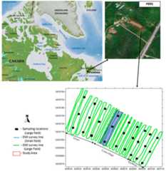
Figure 1. The location of Pynn’s Brook Research Station (PBRS), Pasadena (49°04′20″ N, 57°33′35″ W) in Newfoundland, Canada and the study site.
2.2. SMC Data Recording and TDR Calibration
During the study,SMC was measured using a hand-held time domain reflectometry (TDR) probe. The TDR measuredSMC data were first compared with the calculatedSMC, which was determined by multiplying gravimetricSMC (θg) with the measured average soil bulk density of 1.31 g cm−3. The TDR measuredSMC was compared with the calculatedSMC to evaluate the field scale accuracy of the TDR probe. The average gravimetricSMC, θg (g g−1) was determined for the 0–20 cm (θg(0–20)) depth range by oven drying moist soil samples at 105 °C for 48 h. An integrated TDR, known as HD2-TDR (IMKO Micromodultechnik GmbH, Germany) with probe lengths of 11 cm (θv(0–11)), 16 cm (θv(0–16)) and 30 cm (θv(0–30)) [51] was used. Also, the mean soil temperature measured from the HD2-TDR precision soil moisture probe was used for the temperature conversion of measuredECa data.
2.3. EMI Survey
In this study,ECa was measured using the multi-coil CMD-MINIEXPLORER (GF instruments, Brno, Czech Republic) and the multi-frequency GEM-2 (Geophex, Ltd., Raleigh, NC, USA). The CMD-MINIEXPLORER has 3 coil separations and can be operated at vertical coplanar (VCP) and horizontal coplanar (HCP) coil configurations. The CMD-MINIEXPLORER therefore generates six pseudo depths (PDs), also known as depths of investigation (DOI), of 25, 50 and 90 cm when using VCP modes, and 50, 100, 180 cm when using HCP modes [33]. The theoretical calculation of the DOI for GEM-2 is at a deeper depth compared to the CMD-MINIEXPLORER [52]. However, the accuracy of the DOI of GEM-2 with varying frequencies under heterogenic field conditions is yet to be determined. Based on the preliminary data obtained on the site, the CMD-MINIEXPLORER with the largest coil separation (coil 3 = 118 cm) with PDs of 90 and 180 for VCP and HCP modes, respectively, and a 38 kHz frequency of GEM-2 (the coil separation is 166 cm) were employed in this study. The CMD-MINIEXPLORER at the VCP configuration is represented withECa-L and at the HCP configuration is represented withECa-H while GEM-2 at the HCP configuration is represented withECa-38 kHz. Surveys with CMD-MINIEXPLORER were conducted at a height of 15 cm. The GEM-2 device was carried with the supplied shoulder strap at an average height of 100 cm.
Several studies suggested temperature conversion of rawECa to a standard soil temperature (25 °C) e.g., [1,53] using: whereECt is theECa data collected at measured soil temperature (°C) andEC25 is the temperature correctedECa.
EC25 = ECt × (0.4470 + 1.4034 e−t/26.815)
To avoid data shifts, both sensors were allowed a warm up period of at least 30 min before measurements were recorded [54]. However, no instrumental drift was expected in theECa due to the high temperature stability of the CMD-MINIEXPLORER and GEM-2 [37,55].
EMI surveys were conducted on a small field (45 m × 8.5 m) and a large field (0.45 ha) using CMD-MINIEXPLORER and GEM-2. The large field comprises of the grass, silage-corn and soybean plots while the small field is a portion of the silage-corn experimental plot selected for a detailed field study (Figure 1). TheECa measurements were carried out on 30 September, 6 October, and 18 November in Fall 2016, and on 31 May in Spring 2017. The relationship between CMD-MINIEXPLORER and GEM-2 was assessed by comparing the patterns and trends of measuredECa data from both instruments using a 45 m linear transect collected on 30 September on the small field.
2.4. Field Calibration and Validation
The small field was used to calibrate and validate the relationship betweenSMC andECa using data collected on 30 September and 6 October 2016, respectively. The calibration was carried out using theECa data (ECa-L,ECa-H andECa-38 kHz) and measuredSMC data collected with the HD2-TDR probes (0–11, 0–16, and 0–30 cm) on 30 September 2016. The validation was then carried out using theECa data and HD2-TDR measuredSMC at 0–11 and 0–16 cm depths on 6 October 2016. The validation was further carried out on a 30 m transect on the silage-corn plot and the grass plot at the study site using the data collected on 31 May 2017. The small field survey was carried out on a gridded plot (without GPS) for constant precise point calibration and validation. The proximally sensedECa was determined using the meanECa measurements (n = 20) generated on the small field from CMD-MINIEXPLORER and GEM-2 survey data collected on the same day along each of the selected twenty sampling locations similar to Zhu et al. [56].
To testECa response toSMC variability at a larger spatial scale, a large field study was conducted to validate the regression model generated from the small field on 18 November 2016. The EMI survey on the large field was carried out by walking across the entire field with a GPS connected to CMD-MINIEXPLORER and GEM-2 to obtain geo-referencedECa data. Also, twenty-seven geo-referencedSMC data points (θv(0–16)) were collected using the HD2-TDR 0–16 cm length probe only and a hand held GPS according to the stratified sampling locations.
2.5. Soil Sampling
The silage-corn trial on the small field consisted of 4 m × 1 m plots that received different nutrient management treatments using biochar (BC), dairy manure (DM), inorganic fertilizer, or a combination of these. Soil samplings on the small field were done by selecting twenty sampling locations based on the BC and DM application, though the treatment effects were not significant across the small field [28]. Soil samples were collected from the depths of 0–10 cm and 10–20 cm using a gouge auger and a hammer. Samples were placed in airtight bags and stored in a polystyrene cooler until gravimetricSMC (θg) measurements were carried out in the laboratory.
2.6. Data Analysis
Descriptive statistics (min, max, mean, median, skewness, kurtosis and coefficient of variation, CV) were carried out to evaluate the EMI data andSMC data. Paired samplet-tests were carried out to determine if there were any statistically significant differences between theECa andSMC means. Pearson’s correlation coefficients (r) were used to establish the relationship betweenECa data andSMC data. The coefficient of determination (R2) was used to evaluate the relationship among EMI results. The root mean square error (RMSE) was used to evaluate the accuracy of the HD2-TDR measuredSMC. The root mean square error of prediction (RMSEP) was used to estimate the accuracy of predictedSMC using theECa and TDR measuredSMC data. A simple linear regression was used to evaluate the relationship betweenECa andSMC data. All analyses were performed with Minitab 17 (Minitab 17 Statistical Software, 2010) andECa maps were generated using Surfer 8 (Golden Software, 2002).
3. Results
3.1. SMC Results
A good match between the measuredSMC (θv) from HD2-TDR and the calculatedSMC (θv) by using gravimetricSMC (θg) was obtained, with anR2 of >0.88 and aRMSE < 0.04 m3 m−3 for all three TDR probe lengths (Figure 2 andTable 1). Accuracy of the HD2-TDR for the 16 cm probe length is similar to theRMSE of 0.013 m3 m−3 by Topp et al. [11] while the HD2-TDR for the 11 and 30 cm probe lengths hasRMSE values of 0.040 m3 m−3 and 0.018 m3 m−3, respectively (Figure 2 andTable 1).
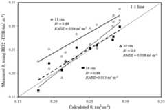
Figure 2. Comparison of the measured θv using the HD2-TDR and calculated θv by using the measured θg and bulk density at Pynn’s Brook Research Station.

Table 1. Linear regression, coefficient of determination (R2) and root mean square error (RMSE) for HD2-TDR calibration at Pynn’s Brook Research Station using the calculated θv from θg (n = 10).
3.2. EMI Results
TheECa patterns and trends along the 45 m transect on the small field were similar for CMD-MINIEXPLORER and GEM-2, despite different DOIs (Figure 3 andFigure 4). The data from CMD-MINIEXPLORER plotted against the GEM-2 data (Figure 5) show thatECa values ofECa-H are closely associated to that of GEM-2 (R2 = 0.71) compared toECa-L (R2 = 0.40). The possibility of integrating the meanECa measurements from the CMD-MINIEXPLORER and the GEM-2 was evaluated with the average ofECa-L,ECa-H andECa-38 kHz and analysed using the backward stepwise multiple linear regression (MLR). The results indicated that they were redundant.
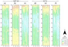
Figure 3. Results of small field EMI surveys on 30 September and 6 October 2016 forECa-L (a,d),ECa-H (b,e) andECa-38 kHz (c,f).
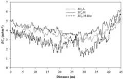
Figure 4. Variability of the measuredECa by the two EMI sensors on a 45 m linear transect in the small field.

Figure 5. Scatter-plot ofECa measured using CMD-MINIEXPLORER and GEM-2.
3.3. Basic Statistics
The descriptive statistics of theECa measurements from CMD-MINIEXPLORER, GEM-2 and the TDR measuredSMC in the study site are given inTable 2. According to the classification of Warrick and Nielsen [57], CVs of CMD-MINIEXPLORER were low (CV < 12%) while those of GEM-2 were moderate (12% < CV < 62%). The CVs of TDR measuredSMC were moderate (CV > 12%) except for the θv(0–11) depth, which was low (Table 2).
Table 2. Descriptive statistics of theECa (mS m−1) measurements using CMD-MINIEXPLORER and GEM-2 and TDR measuredSMC (m3 m−3) at the study site (n = 20).
A paired samplet-test was performed using a sample of 20ECa data points from the small field to determine whether there was a difference between means ofECa from CMD-MINIEXPLORER and GEM-2. Results revealed thatECa means ofECa-38 kHz (3.214 ± 0.718) were significantly different fromECa-L (3.576 ± 0.323) andECa-H (4.139 ± 0.466), withp = 0.050 andp = 0.000, respectively.
A paired samplet-test was also carried out on a sample of 20SMC data points to determine whether there was a difference in theSMC means at different depths. TheSMC mean for θv(0–11) (0.28755 ± 0.03241) was significantly different from the means obtained for θv(0–16) (0.25268 ± 0.03690) and θv(0–30) (0.2471 ± 0.0507); both differences had the samep = 0.000. Pearson’s correlation coefficients amongECa measurements andSMC are shown inTable 3. At ap-value < 0.1,ECa data (CMD-MINIEXPLORER and GEM-2) were significantly correlated withSMC measurements.
Table 3. Pearson’s correlation coefficients of theECa measurements of CMD-MINIEXPLORER and GEM-2 and TDR measuredSMC at the study site (n = 20). Significance is reported at the 0.1 (*), 0.05 (**), and 0.001 (***)p-values.
3.4. Regression Analysis
The fitted linear regressions (LRs) to estimateSMC for different integral depths using measuredECa with CMD-MINIEXPLORER or GEM-2 data are shown inFigure 6 and respective statistics for calibration and validation betweenECa and TDR measuredSMC are summarized inTable 4. TheSMC estimates obtained usingECa-L (R2p = 0.38 and 0.54) are better than the estimates forECa-H andECa-38 kHz, withRMSEP 0.033 and 0.031 m3 m−3, respectively (Table 4).
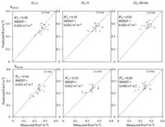
Figure 6. Plots of predicted θv (m3 m−3) usingECa data versus TDR measured θv (m3 m−3) for the linear regressions given inTable 4 forECa-L,ECa-H andECa-38 kHz.
Table 4. Linear regressions betweenECa data from CMD-MINIEXPLORER and GEM-2 with TDR measuredSMC for different integral depths (n = 20).
Because the purpose of the large field study was to evaluate theECa response to variability inSMC at a larger spatial scale, only the θv(0–16) depth with the highest accuracy for the study site (Table 1) was measured at 27 geo-referenced locations on the field. The linear regression between θv(0–16) andECa-L on the small field was used for the large field study. The estimates ofSMC for θv(0–16) usingECa-L were lower for the large field study than for the small field study (RMSEP = 0.076 m3 m−3).
The same linear regressions were applied to a 30 m transect in the corn-silage plot and the grass plot at the study site (Table 5) for validation of linear regressions. The estimates ofSMC viaECa-L for the grass plot had lowerR2 values (from 0.07 to 0.32) and higherRMSEP (from 0.039 to 0.074 m3 m−3) than for the silage-corn plot (R2 = from 0.30 to 0.59;RMSEP = from 0.041 to 0.072 m3 m−3). Overall, fitted linear regressions developed betweenECa andSMC in this study have shown higher prediction accuracy forECa-L than forECa-H andECa-38 kHz.
Table 5. Validation of the fitted linear regressions summarised inTable 4, usingECa data from CMD-MINIEXPLORER and GEM-2 with TDR measuredSMC on a 30 m transect (n = 11).
3.5. ECa Mapping
The spatial variability ofECa was mapped across the study site by variogram analysis and ordinary block kriging using Surfer 8 (Golden Software, 2002, Golden, CO, USA). The trends ofECa data from the CMD-MINIEXPLORER and the GEM-2 show similar patterns despite different DOIs (or sampling volume) andECa values (Figure 7). For instance, largerECa values were measured at the northwest and southeast sections of the study site while lowerECa values were found on the northeast section, which stretches across the middle area of the field. The map ofSMC predicted using theECa-L and the 27 georeferenced measurements (Figure 8) shows similar patterns with lower values (<0.28 m3 m−3) across the centre of the study site.
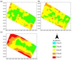
Figure 7. Spatial variability maps ofECa for the large field study (a)ECa-L (b)ECa-H (c)ECa-38 kHz.
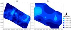
Figure 8. Spatial variability maps ofSMC for the large field study estimated usingECa-L measurements (a) and 27 geo-referenced point measurements using the HD2-TDR (b).
4. Discussion
The factory calibration of HD2-TDR is not sufficient for field applications as it was carried out in a repacked soil with uniform temperature and low bulk electrical conductivity [51]. Also, a low representative elemental volume of soils, which affects the variability of moisture content, has been reported for many current sensor technologies as well as direct sampling methods [58]. This variability has been attributed to several factors such as gravel content and position in the landscape, which influences water content variation across the field [58]. In this study, visual observations indicated a highly disturbed soil surface and high gravel content at the 0–10 cm soil depth and positions of measurement (point measurements) within the study area. This may be assumed to have led to differences between the 11 cm HD2-TDR probe data and the calculatedSMC from the gravimetricSMC (Figure 2). This behaviour implies that it is not a field error (Std Dev = 0.037 m3 m−3), but a high spatial variability of the field water content within the shallow depth.
Khan et al. [43] reported a lowECa, between 2.1 and 35.5 mS m−1, on an orthic Humo-ferric podzol while Pan et al. [59] indicated a lowECa between 1.36 and 3.29 mS m−1 in a sandy soil. Martini et al. [60] also observed a lowECa, between 0 and 24 mS m−1, with a very small range of spatial variation which was predominantly attributed to the low heterogeneity of soil texture (Sand = 6%–28%, Silt = 55%–79%, Clay = 13%–25%). TheseECa ranges of previous studies are similar to the results of our study site, classified as an orthic Humo-ferric podzol, with a lowerECa ranging between 0 and 7 mS m−1 and also with a low textural variation (Sand = 80.10%–83.75%, Silt = 10.44%–12.58%, Clay = 5.81%–7.32%). Although the report by Martini et al. [60] has low sand content and variation, the clay content (which is one of the factors that can influenceECa; McNeill [20]) is lower at both sites of this study.
The depth range (0–20 cm) considered in this study, also includes the Podzolic Ae horizon with a texture that is coarser than the adjacent horizons [44]. The known depth-response function of CMD-MINIEXPLORER has been used by various authors to calibrate the sensor, even though not all coil separations exhibit low signal to noise levels [33,61].
Arguably, the multi-frequency GEM-2 sensor measures at a deeper DOI compared to the multi-coil CMD-MINIEXPLORER sensor. The measuredECa from the GEM-2 sensor has lower values compared to the measuredECa from the CMD-MINIEXPLORER sensor with known DOIs of 90 cm and 180 cm for low (ECa-L) and high (ECa-H) coil 3 dipole configurations, respectively. Evaluating theECa measurements by GEM-2 with the site soil and parent material using the EMI skin depth, Nomogram [52] also confirmed a greater DOI than 180 cm. When the DOI increases, weaker signals indicate a less conductive soil, whereby stronger signals are observed with decreasing DOI [38,39]. Additionally, the CMD-MINIEXPLORER with the coil 3 dipole configuration adopted in this study shows the highest local sensitivity at a depth between 0–35 cm and 0–75 cm, according to the sensitivity function by McNeil [20]. This provides a reasonable match between the sensing volume of EMI and the depth range sampled by the HD2-TDR precision soil moisture probe, considering the DOI from the soil surface as zero. The largest coil separation in VCP mode was also less sensitive to variations in instrument height that inevitably occurred when EMI measurements were carried out.
Warrick and Nielsen [57] proposed the use of CV categories, which have been widely adopted to assess the soil’s spatial variability. This procedure allows for comparisons across samples that employ different units of measurement [62]. However, the geostatistical techniques must be carried out to understand the spatial dependence among the variables [63]. Molin and Faulin [64] found CVs forECa andSMC to be moderate (43% and 57%). These findings are similar to the results of this study even though CVs are less than 23% (Table 2). The CVs ofECa-L,ECa-H, andECa-38 kHz measurements and measuredSMC (Table 2) suggest thatECa values respond to vertical heterogeneity of soil properties [65] such asSMC variability along the soil depth.
Other researchers also found considerable site-to-site variability in the relationship betweenECa andSMC e.g., [25], similar to our study. TheR2 andRMSE of validation models are not consistent when compared to those of calibration models (Table 4). For instance, calibration using θv(0–16) produced anR2 of 0.74 andRMSE of 0.018 m3 m−3 while validation producedR2 of 0.54 andRMSEP of 0.031 m3 m−3. TheR2 generated when the detailed field study regression models were applied to the grass plot showed a need for site-specific calibration to establish the relationship betweenECa andSMC (Table 5). Also, theR2 and theRMSE values forSMC presented inFigure 6 forECa-L,ECa-H, andECa-38 kHz measurements vary by 0.031 m3 m−3 and 0.040 m3 m−3. This implies that the variation inSMC can be attributed to the maximum sensitivity of theECa.
Martini et al. [60] observed thatSMC monitoring usingECa requires the determination of the temporal variations of all other variables that can induceECa (e.g., temperature andECw) while Altdorff et al. [66] reported that EMI has the potential to account for a strong influence ofSMC onECa. Even though our study did not account for all variables, the data set used in this study gave a reasonably accurate site-specific calibration ofSMC at the study site. However, spatial statistics techniques such as variogram modelling are needed to confirm the number of required sampling points and capture the spatial variability more accurately.
This study confirms the relationship betweenECa andSMC through the correlation between the spatial pattern ofECa (Figure 7) andSMC (Figure 8). Regions of lowECa correspond to regions of lowSMC and vice versa. For instance, the region with theECa > 5 mS m−1 corresponds to theSMC region > 0.28 m3 m−3 and the region withECa < 4 mS m−1 corresponds to theSMC region < 0.23 m3 m−3. The spatial variability of geo-referencedSMC is lower thanECa-L predictedSMC (Figure 8), as expected. This may indicate the need for more sampling locations to fully capture the spatial variability ofSMC and its effects on the map interpolation.
5. Conclusions
Analysis of the relationships betweenECa measurements using two EMI sensors (CMD-MINIEXPLORER and GEM-2), andSMC using oven drying and HD2-TDR methods were carried out on a podzolic soil at an experimental site in western Newfoundland, Canada. Linear regression analysis used to estimateSMC from the two EMI sensors usingECa data at the study site provided the best prediction forSMC at 0–11 cm and 0–16 cm depth ranges.
The validation results show that to derive reasonably accurate regression models for predictingSMC from EMI measurements for field scale mapping ofSMC, sitespecific calibration is required. The site-specific calibration ofECa-SMC can be determined using linear regression models. This can be attributed to the potential of CMD-MINIEXPLORER and GEM-2 to measure the strong influence ofSMC onECa implying that theSMC is a major driver ofECa measurement at the study site.
A good relationship was found between the measuredECa from CMD-MINIEXPLORER and GEM-2 at the study site. The CMD-MINIEXPLORER and GEM-2 were observed to have similar values for the selected coil orientation and frequency used in this study. Though the temperature effect is minimal, it is important to conduct the direct measurements and EMI measurements from the two EMI sensors within a short period of time as there will be minor changes ofSMC.
Further research on the prediction of profile depth and sampling volume at the field needs to be conducted to confirm ifSMC is the basic driver of CMD-MINIEXPLORER and GEM-2 response along the depth and horizontal variation at a large scale.
Author Contributions
Conceptualization, L.G.; Data curation, E.B. and L.G.; Formal analysis, E.B.; Funding acquisition, L.G.; Investigation, E.B.; Methodology, E.B. and L.G.; Project administration, L.G.; Resources, M.C., V.K. and L.G.; Supervision, A.U. and L.G.; Writing—original draft, E.B.; Writing—review & editing, A.U., M.C., V.K. and L.G.
Funding
This research was funded by Research and Development Corporation of Newfoundland and Labrador throughIgnite R&D program 5404-1962-101 and the Research Office of Grenfell Campus, Memorial University of Newfoundland through stat-up fund 20160160.
Acknowledgments
We acknowledge an MSc—BEAS graduate fellowship from Memorial University, E. Badewa, and data-collection support by Marli Vermooten, Dinushika Wanniarachchi and Kamaleswaran Sadatcharam.
Conflicts of Interest
The authors declare no conflict of interest. The funders had no role in the design of the study; in the collection, analyses, or interpretation of data; in the writing of the manuscript, and in the decision to publish the results.
References
- Corwin, D.L.; Lesch, S.M. Characterizing soil spatial variability with apparent soil electrical conductivity part II. case study.Comput. Electron. Agric.2005,46, 135–152. [Google Scholar] [CrossRef]
- Peralta, N.R.; Costa, J.L. Delineation of management zones with soil apparent electrical conductivity to improve nutrient management.Comput. Electron. Agric.2013,99, 218–226. [Google Scholar] [CrossRef]
- Lesch, S.M.; Corwin, D.L.; Robinson, D.A. Apparent soil electrical conductivity mapping as an agricultural management tool in arid zone soils.Comput. Electron. Agric.2005,46, 351–378. [Google Scholar] [CrossRef]
- Bongiovanni, R.; Lowenberg-DeBoer, J. Precision agriculture and sustainability.Precis. Agric.2004,5, 359–387. [Google Scholar] [CrossRef]
- Kyaw, T.; Ferguson, R.B.; Adamchuk, V.I.; Marx, D.B.; Tarkalson, D.D.; McCallister, D.L. Delineating site-specific management zones for pH-induced iron chlorosis.Precis. Agric.2008,9, 71–84. [Google Scholar] [CrossRef]
- Fortes, R.; Millán, S.; Prieto, M.H.; Campillo, C. A methodology based on apparent electrical conductivity and guided soil samples to improve irrigation zoning.Precis. Agric.2015,16, 441–454. [Google Scholar] [CrossRef]
- Corwin, D.L.; Lesch, S.M. Apparent soil electrical conductivity measurements in agriculture.Comput. Electron. Agric.2005,46, 11–43. [Google Scholar] [CrossRef]
- Doolittle, J.A.; Brevik, E.C. The use of electromagnetic induction techniques in soils studies.Geoderma2014,223, 33–45. [Google Scholar] [CrossRef]
- Galagedara, L.W.; Parkin, G.W.; Redman, J.D.; von Bertoldi, P.; Endres, A.L. Field studies of the GPR ground wave method for estimating soil water content during irrigation and drainage.J. Hydrol.2005,301, 182–197. [Google Scholar] [CrossRef]
- Wijewardana, Y.G.N.S.; Galagedara, L.W. Estimation of spatio-temporal variability of soil water content in agricultural fields with ground penetrating radar.J. Hydrol.2010,391, 24–33. [Google Scholar] [CrossRef]
- Topp, G.C.; Davis, J.L.; Annan, A.P. Electromagnetic determination of soil water content: Measurements in coaxial transmission lines.Water Resour. Res.1980,16, 574–582. [Google Scholar] [CrossRef]
- Ferré, P.A.; Redman, J.D.; Rudolph, D.L.; Kachanoski, R.G. The dependence of the electrical conductivity measured by time domain reflectometry on the water content of a sand.Water Resour. Res.1998,34, 1207–1213. [Google Scholar] [CrossRef]
- Desilets, D.; Zreda, M.; Ferre, T.P.A. Nature’s neutron probe: Land surface hydrology at an elusive scale with cosmic rays.Water Resour. Res.2010. [Google Scholar] [CrossRef]
- Franz, T.E.; Zreda, M.; Ferre, P.A.; Rosolem, R. An assessment of the effect of horizontal soil moisture heterogeneity on the area-average measurement of cosmic-ray neutrons.Water Resour. Res.2013,49, 1–10. [Google Scholar] [CrossRef]
- Mondal, P.; Tewari, V.K. Present status of precision farming: A review.Int. J. Agric. Res.2007,5, 1124–1133. [Google Scholar]
- Jay, S.C.; Lawrence, R.L.; Repasky, K.S.; Rew, L.J. Detection of leafy spurge using hyper-spectral-spatial-temporal imagery. In Proceedings of the 2010 IEEE International Geoscience and Remote Sensing Symposium, Honolulu, HI, USA, 25–30 July 2010; IEEE: Bozeman, MT, USA; pp. 4374–4376. [Google Scholar]
- Zhang, Z.; He, G.; Jiang, H. Leaf area index retrieval using red edge parameters based on Hyperion hyper-spectral imagery.J. Theor. Appl. Inf. Technol.2013,48, 957–960. [Google Scholar]
- Rudolph, S.; van der Kruk, J.; von Hebel, C.; Ali, M.; Herbst, M.; Montzka, C.; Pätzold, S.; Robinson, D.A.; Vereecken, H.; Weihermüller, L. Linking satellite derived LAI patterns with subsoil heterogeneity using large-scale ground-based electromagnetic induction measurements.Geoderma2015,241–242, 262–271. [Google Scholar] [CrossRef]
- Rhoades, J.D.; Raats, P.A.; Prather, R.J. Effects of liquid-phase electrical conductivity, water content, and surface conductivity on bulk soil electrical conductivity.Soil Sci. Soc. Am. J.1976,40, 651–655. [Google Scholar] [CrossRef]
- McNeill, J.D.Electromagnetic Terrain Conductivity Measurement at Low Induction Numbers; Geonics Ltd.: Mississauga, ON, Canada, 1980. [Google Scholar]
- Kachanoski, R.G.; Gregorich, E.G.; van Wesenbeeck, I.J. Estimating spatial variations of soil water content using non contacting electromagnetic inductive methods.Can. J. Soil Sci.1988,68, 715–722. [Google Scholar] [CrossRef]
- Brevik, E.C.; Fenton, T.E. The relative influence of soil water, clay, temperature, and carbonate minerals on soil electrical conductivity readings with an EM-38 along a Mollisol catena in central Iowa.Soil Surv. Horiz.2002,43, 9–13. [Google Scholar] [CrossRef]
- Corwin, D.L.; Lesch, S.M. Application of soil electrical conductivity to precision agriculture.Agron. J.2003,95, 455–471. [Google Scholar] [CrossRef]
- Friedman, S.P. Soil properties influencing apparent electrical conductivity: A review.Comput. Electron. Agric.2005,46, 45–70. [Google Scholar] [CrossRef]
- Brevik, E.C.; Fenton, T.E.; Lazari, A. Soil electrical conductivity as a function of soil water content and implications for soil mapping.Precis. Agric.2006,7, 393–404. [Google Scholar] [CrossRef]
- Serrano, J.M.; Shahidian, S.; da Silva, J.R.M. Apparent electrical conductivity in dry versus wet soil conditions in a shallow soil.Precis. Agric.2013,14, 99–114. [Google Scholar] [CrossRef]
- Huang, J.; Scudiero, E.; Bagtang, M.; Corwin, D.L.; Triantafilis, J. Monitoring scale-specific and temporal variation in electromagnetic conductivity images.Irrig. Sci.2016,34, 187–200. [Google Scholar] [CrossRef]
- Altdorff, D.; Galagedara, L.; Nadeem, M.; Cheema, M.; Unc, A. Effect of agronomic treatments on the accuracy of soil moisture mapping by electromagnetic induction.Catena2018,164, 96–106. [Google Scholar] [CrossRef]
- Lesch, S.M.; Strauss, D.J.; Rhoades, J.D. Spatial prediction of soil salinity using electromagnetic induction techniques. Part 1. Statistical prediction models: A comparison of multiple linear regression and cokriging.Water Resour. Res.1995,31, 373–386. [Google Scholar] [CrossRef]
- Goff, A.; Huang, J.; Wong, V.N.L.; Monteiro Santos, F.A.; Wege, R.; Triantafilis, J. Electromagnetic conductivity imaging of soil salinity in an estuarine–Alluvial landscape.Soil Sci. Soc. Am. J.2014,78, 1686. [Google Scholar] [CrossRef]
- Lesch, S.M.; Corwin, D.L. Predicting EM/soil property correlation estimates via the dual pathway parallel conductance model.Agron. J.2003,95, 365–379. [Google Scholar] [CrossRef]
- Walter, J.; Lueck, E.; Bauriegel, A.; Richter, C.; Zeitz, J. Multi-scale analysis of electrical conductivity of peatlands for the assessment of peat properties.Eur. J. Soil Sci.2015,66, 639–650. [Google Scholar] [CrossRef]
- Altdorff, D.; Bechtold, M.; van der Kruk, J.; Vereecken, H.; Huisman, J.A. Mapping peat layer properties with multi-coil offset electromagnetic induction and laser scanning elevation data.Geoderma2016,261, 178–189. [Google Scholar] [CrossRef]
- Bittelli, M. Measuring soil water content: A review.HortTechnology2011,21, 293–300. [Google Scholar]
- Huang, J.; Nhan, T.; Wong, V.N.L.; Johnston, S.G.; Lark, R.M.; Triantafilis, J. Digital soil mapping of a coastal acid sulfate soil landscape.Soil Res.2014,52, 327–339. [Google Scholar] [CrossRef]
- Vereecken, H.; Huisman, J.A.; Pachepsky, Y.; Montzka, C.; Van Der Kruk, J.; Bogena, H.; Weihermüller, L.; Herbst, M.; Martinez, G.; Vanderborght, J. On the spatio-temporal dynamics of soil moisture at the field scale.J. Hydrol.2014,516, 76–96. [Google Scholar] [CrossRef]
- Allred, B.J.; Ehsani, M.R.; Saraswat, D. The impact of temperature and shallow hydrologic conditions on the magnitude and spatial pattern consistency of electromagnetic induction measured soil electrical conductivity.Am. Soc. Agric. Eng.2005,48, 2123–2135. [Google Scholar] [CrossRef]
- Callegary, J.B.; Ferré, T.P.A.; Groom, R.W. Vertical spatial sensitivity and exploration depth of low-induction-number electromagnetic induction instruments.Vadose Zone J.2007,6, 158–167. [Google Scholar] [CrossRef]
- Delefortrie, S.; Saey, T.; Van De Vijver, E.; De Smedt, P.; Missiaen, T.; Demerre, I.; Van Meirvenne, M. Frequency domain electromagnetic induction survey in the intertidal zone: Limitations of low-induction-number and depth of exploration.J. Appl. Geophys.2014,100, 14–22. [Google Scholar] [CrossRef]
- Horney, R.D.; Taylor, B.; Munk, D.S.; Roberts, B.A.; Lesch, S.M.; Plant, R.E. Development of practical site-specific management methods for reclaiming salt-affected soil.Comput. Electron. Agric.2005,46, 379–397. [Google Scholar] [CrossRef]
- Triantafilis, J.; Terhune IV, C.H.; Monteiro Santos, F.A. An inversion approach to generate electromagnetic conductivity images from signal data.Environ. Model. Softw.2013,43, 88–95. [Google Scholar] [CrossRef]
- Singh, G.; Williard, K.W.; Schoonover, J.E. Spatial relation of apparent soil electrical conductivity with crop yields and soil properties at different topographic positions in a small agricultural watershed.Agronomy2016,6, 57. [Google Scholar] [CrossRef]
- Khan, F.S.; Zaman, Q.U.; Chang, Y.K.; Farooque, A.A.; Schumann, A.W.; Madani, A. Estimation of the rootzone depth above a gravel layer (in wild blueberry fields) using electromagnetic induction method.Precis. Agric.2016,17, 155–167. [Google Scholar] [CrossRef]
- Soil Classification Working Group.The Canadian System of Soil Classification, 3rd ed.; Agriculture and Agri-Food Canada Publication: Ottawa, ON, Canada, 1998. [Google Scholar]
- Driessen, P.; Deckers, J.; Spaargaren, O.; Nachtergaele, F.Lecture Notes on the Major Soils of the World; Food and Agriculture Organization of the United Nations (FAO): Rome, Italy, 2001. [Google Scholar]
- Sanborn, P.; Lamontagne, L.; Hendershot, W. Podzolic soils of Canada: Genesis, distribution, and classification.Can. J. Soil Sci.2011,91, 843–880. [Google Scholar] [CrossRef]
- King, M.; Altdorff, D.; Li, P.; Galagedara, L.; Holden, J.; Unc, A. Northward shift of the agricultural climate zone under 21st-century global climate change.Sci. Rep.2018. [Google Scholar] [CrossRef] [PubMed]
- Wang, C.; Rees, H.W.; Daigle, J.L. Classification of podzolic soils as affected by cultivation.Can. J. Soil Sci.1984,64, 229–239. [Google Scholar] [CrossRef]
- Altdorff, D.; Galagedara, L.; Unc, A. Impact of projected land conversion on water balance of boreal soils in western Newfoundland.J. Water Clim. Chang.2017. [Google Scholar] [CrossRef]
- Kirby, G.E. In Soils of the Pasadena-Deer Lake Area, Newfoundland. 1988. Available online:http://sis.agr.gc.ca/cansis/publications/surveys/nf/nf17/nf17_report.pdf (accessed on 7 November 2016).
- IMKO. TRIME-TDR User Manual. Available online:https://imko.de/en/about-trime-tdr (accessed on 8 December 2016).
- Won, I.J. A wide-band electromagnetic exploration method—Some theoretical and experimental results.Geophysics1980,45, 928–940. [Google Scholar] [CrossRef]
- Ma, R.; McBratney, A.; Whelan, B.; Minasny, B.; Short, M. Comparing temperature correction models for soil electrical conductivity measurement.Precis. Agric.2011,12, F55–F66. [Google Scholar] [CrossRef]
- Robinson, D.A.; Lebron, I.; Lesch, S.M.; Shouse, P. Minimizing drift in electrical conductivity measurements in high temperature environments using the EM-38.Soil Sci. Soc. Am. J.2004,68, 339–345. [Google Scholar] [CrossRef]
- GF Instruments. CMD Electromagnetic Conductivity Meter User Manual V. 1.5. Geophysical Equipment and Services, Czech Republic, 2011. Available online:http://www.gfinstruments.cz/index.php?menu=gi&smenu=iem&cont=cmd_&ear=ov (accessed on 4 June 2016).
- Zhu, Q.; Lin, H.; Doolittle, J. Repeated electromagnetic induction surveys for determining subsurface hydrologic dynamics in an agricultural landscape.Soil Sci. Soc. Am. J.2010,74, 1750–1762. [Google Scholar] [CrossRef]
- Warrick, A.W.; Nielsen, D.R. Spatial variability of soil physical properties in the field. InApplications of Soil Physics; Hillel, D., Ed.; Academic Press: New York, NY, USA, 1980; pp. 319–344. [Google Scholar]
- Hignett, C.; Evett, S. Direct and Surrogate Measures of Soil Water Content. International Atomic Energy Agency, Soil and Water Management and Crop Nutrition Section, Vienna (Austria). No. IAEA-TCS-30. 2008. Available online:http://www-pub.iaea.org/MTCD/publications/PDF/TCS-30_web.pdf (accessed on 8 September 2016).
- Pan, L.; Adamchuk, V.I.; Prasher, S.; Gebbers, R.; Taylor, R.S.; Dabas, M. Vertical soil profiling using a galvanic contact resistivity scanning approach.Sensors2014,14, 13243–13255. [Google Scholar] [CrossRef] [PubMed]
- Martini, E.; Werban, U.; Zacharias, S.; Pohle, M.; Dietrich, P.; Wollschläger, U. Repeated electromagnetic induction measurements for mapping soil moisture at the field scale: Validation with data from a wireless soil moisture monitoring network.Hydrol. Earth Syst. Sci.2017,21, 495. [Google Scholar] [CrossRef]
- Bonsall, J.; Fry, R.; Gaffney, C.; Armit, I.; Beck, A.; Gaffney, V. Assessment of the CMD mini-explorer, a new low-frequency multi-coil electromagnetic device, for archaeological investigations.Archaeol. Prospect.2013,20, 219–231. [Google Scholar] [CrossRef]
- Souza, Z.M.D.; Marques Júnior, J.; Pereira, G.T. Spatial variability of the physical and mineralogical properties of the soil from the areas with variation in landscape shapes.Braz. Arch. Biol. Technol.2009,52, 305–316. [Google Scholar] [CrossRef]
- Liu, T.L.; Juang, K.W.; Lee, D.Y. Interpolating soil properties using kriging combined with categorical information of soil maps.Soil Sci. Soc. Am. J.2006,70, 1200–1209. [Google Scholar] [CrossRef]
- Molin, J.P.; Faulin, G.D.C. Spatial and temporal variability of soil electrical conductivity related to soil moisture.Sci. Agricola2013,70, 1–5. [Google Scholar] [CrossRef]
- Neely, H.L.; Morgan, C.L.; Hallmark, C.T.; McInnes, K.J.; Molling, C.C. Apparent electrical conductivity response to spatially variable vertisol properties.Geoderma2016,263, 168–175. [Google Scholar] [CrossRef]
- Altdorff, D.; von Hebel, C.; Borchard, N.; van der Kruk, J.; Bogena, H.R.; Vereecken, H.; Huisman, J.A. Potential of catchment-wide soil water content prediction using electromagnetic induction in a forest ecosystem.Environ. Earth Sci.2017,76, 111. [Google Scholar] [CrossRef]
Figure 1. The location of Pynn’s Brook Research Station (PBRS), Pasadena (49°04′20″ N, 57°33′35″ W) in Newfoundland, Canada and the study site.
Figure 1. The location of Pynn’s Brook Research Station (PBRS), Pasadena (49°04′20″ N, 57°33′35″ W) in Newfoundland, Canada and the study site.

Figure 2. Comparison of the measured θv using the HD2-TDR and calculated θv by using the measured θg and bulk density at Pynn’s Brook Research Station.
Figure 2. Comparison of the measured θv using the HD2-TDR and calculated θv by using the measured θg and bulk density at Pynn’s Brook Research Station.

Figure 3. Results of small field EMI surveys on 30 September and 6 October 2016 forECa-L (a,d),ECa-H (b,e) andECa-38 kHz (c,f).
Figure 3. Results of small field EMI surveys on 30 September and 6 October 2016 forECa-L (a,d),ECa-H (b,e) andECa-38 kHz (c,f).

Figure 4. Variability of the measuredECa by the two EMI sensors on a 45 m linear transect in the small field.
Figure 4. Variability of the measuredECa by the two EMI sensors on a 45 m linear transect in the small field.

Figure 5. Scatter-plot ofECa measured using CMD-MINIEXPLORER and GEM-2.
Figure 5. Scatter-plot ofECa measured using CMD-MINIEXPLORER and GEM-2.

Figure 6. Plots of predicted θv (m3 m−3) usingECa data versus TDR measured θv (m3 m−3) for the linear regressions given inTable 4 forECa-L,ECa-H andECa-38 kHz.
Figure 6. Plots of predicted θv (m3 m−3) usingECa data versus TDR measured θv (m3 m−3) for the linear regressions given inTable 4 forECa-L,ECa-H andECa-38 kHz.

Figure 7. Spatial variability maps ofECa for the large field study (a)ECa-L (b)ECa-H (c)ECa-38 kHz.
Figure 7. Spatial variability maps ofECa for the large field study (a)ECa-L (b)ECa-H (c)ECa-38 kHz.

Figure 8. Spatial variability maps ofSMC for the large field study estimated usingECa-L measurements (a) and 27 geo-referenced point measurements using the HD2-TDR (b).
Figure 8. Spatial variability maps ofSMC for the large field study estimated usingECa-L measurements (a) and 27 geo-referenced point measurements using the HD2-TDR (b).

Table 1. Linear regression, coefficient of determination (R2) and root mean square error (RMSE) for HD2-TDR calibration at Pynn’s Brook Research Station using the calculated θv from θg (n = 10).
Table 1. Linear regression, coefficient of determination (R2) and root mean square error (RMSE) for HD2-TDR calibration at Pynn’s Brook Research Station using the calculated θv from θg (n = 10).
| SMC | Regression Equation | R2 | RMSE |
|---|---|---|---|
| θv(0–11) | 0.8646 (θv) + 0.0708 | 0.89 | 0.040 |
| θv(0–16) | 0.9330 (θv) + 0.0193 | 0.88 | 0.013 |
| θv(0–30) | 1.2137 (θv) − 0.0462 | 0.90 | 0.018 |
Table 2. Descriptive statistics of theECa (mS m−1) measurements using CMD-MINIEXPLORER and GEM-2 and TDR measuredSMC (m3 m−3) at the study site (n = 20).
Table 2. Descriptive statistics of theECa (mS m−1) measurements using CMD-MINIEXPLORER and GEM-2 and TDR measuredSMC (m3 m−3) at the study site (n = 20).
| Depth | Min | Max | Mean | Median | Skewness | Kurtosis | CV |
|---|---|---|---|---|---|---|---|
| ECa-L | 2.79 | 3.99 | 3.58 a | 3.68 | −0.9 | 0.5 | 9.0 |
| ECa-H | 3.45 | 4.88 | 4.14 a | 4.14 | −0.1 | −1.0 | 11.3 |
| ECa-38 kHz | 2.15 | 4.58 | 3.21 b | 3.2 | 0.2 | −0.9 | 22.4 |
| θv(0–11) | 0.23 | 0.34 | 0.29 c | 0.30 | −0.5 | −0.6 | 11.3 |
| θv(0–16) | 0.16 | 0.31 | 0.25 d | 0.26 | −0.7 | 0.2 | 14.6 |
| θv(0–30) | 0.16 | 0.35 | 0.25 d | 0.26 | 0.1 | −0.4 | 20.5 |
Means that do not share a letter are significantly different at 5% probability.
Table 3. Pearson’s correlation coefficients of theECa measurements of CMD-MINIEXPLORER and GEM-2 and TDR measuredSMC at the study site (n = 20). Significance is reported at the 0.1 (*), 0.05 (**), and 0.001 (***)p-values.
Table 3. Pearson’s correlation coefficients of theECa measurements of CMD-MINIEXPLORER and GEM-2 and TDR measuredSMC at the study site (n = 20). Significance is reported at the 0.1 (*), 0.05 (**), and 0.001 (***)p-values.
| ECa-L | ECa-H | ECa-38 kHz | θv(0–11) | θv(0–16) | θv(0–30) | |
|---|---|---|---|---|---|---|
| ECa-L | 1 | |||||
| ECa-H | 0.88 *** | 1 | ||||
| ECa-38 kHz | 0.63 ** | 0.84 *** | 1 | |||
| θv(0–11) | 0.89 *** | 0.74 *** | 0.54 ** | 1 | ||
| θv(0–16) | 0.86 *** | 0.68 *** | 0.50 ** | 0.95 *** | 1 | |
| θv(0–30) | 0.59 ** | 0.42 * | 0.41 * | 0.75 *** | 0.79 *** | 1 |
Table 4. Linear regressions betweenECa data from CMD-MINIEXPLORER and GEM-2 with TDR measuredSMC for different integral depths (n = 20).
Table 4. Linear regressions betweenECa data from CMD-MINIEXPLORER and GEM-2 with TDR measuredSMC for different integral depths (n = 20).
| ECa | SMC | Regression Equation | Calibration | Validation | ||
|---|---|---|---|---|---|---|
| R2 | RMSE | R2p | RMSEP | |||
| ECa-L | θv(0–11) | 0.0888ECa-L − 0.0301 | 0.79 | 0.015 | 0.38 | 0.033 |
| θv(0–16) | 0.0983ECa-L − 0.0988 | 0.74 | 0.018 | 0.54 | 0.031 | |
| θv(0–30) | 0.0925ECa-L − 0.0836 | 0.35 | 0.040 | - | - | |
| ECa-H | θv(0–11) | 0.0515ECa-H + 0.0743 | 0.55 | 0.021 | 0.15 | 0.032 |
| θv(0–16) | 0.0542ECa-H + 0.0284 | 0.47 | 0.026 | 0.32 | 0.031 | |
| θv(0–30) | 0.0462ECa-H + 0.056 | 0.18 | 0.045 | - | - | |
| ECa-38 kHz | θv(0–11) | 0.0243ECa-38 kHz + 0.2095 | 0.29 | 0.027 | 0.01 | 0.036 |
| θv(0–16) | 0.0257ECa-38 kHz + 0.1701 | 0.25 | 0.031 | 0.05 | 0.040 | |
| θv(0–30) | 0.0292ECa-38 kHz + 0.1533 | 0.17 | 0.045 | - | - | |
Table 5. Validation of the fitted linear regressions summarised inTable 4, usingECa data from CMD-MINIEXPLORER and GEM-2 with TDR measuredSMC on a 30 m transect (n = 11).
Table 5. Validation of the fitted linear regressions summarised inTable 4, usingECa data from CMD-MINIEXPLORER and GEM-2 with TDR measuredSMC on a 30 m transect (n = 11).
| SMC | ECa | Silage Corn Plot | Grass Plot | ||
|---|---|---|---|---|---|
| R2p | RMSEP | R2p | RMSEP | ||
| θv(0–11) | ECa-L | 0.30 | 0.046 | 0.13 | 0.066 |
| ECa-H | 0.35 | 0.054 | 0.32 | 0.062 | |
| ECa-38 kHz | 0.30 | 0.041 | 0.30 | 0.074 | |
| θv(0–16) | ECa-L | 0.55 | 0.070 | 0.07 | 0.071 |
| ECa-H | 0.58 | 0.044 | 0.26 | 0.053 | |
| ECa-38 kHz | 0.59 | 0.072 | 0.23 | 0.061 | |
| θv(0–30) | ECa-L | - | - | 0.07 | 0.062 |
| ECa-H | - | - | 0.18 | 0.039 | |
| ECa-38 kHz | - | - | 0.14 | 0.040 | |
© 2018 by the authors. Licensee MDPI, Basel, Switzerland. This article is an open access article distributed under the terms and conditions of the Creative Commons Attribution (CC BY) license (http://creativecommons.org/licenses/by/4.0/).
Article Metrics
Citations
Article Access Statistics
Multiple requests from the same IP address are counted as one view.