lsim#

scipy.signal.lsim(system,U,T,X0=None,interp=True)[source]#

Simulate output of a continuous-time linear system.

Parameters:

systeman instance of the LTI class or a tuple describing the system.

The following gives the number of elements in the tuple andthe interpretation:

• 1: (instance oflti)

• 2: (num, den)

• 3: (zeros, poles, gain)

• 4: (A, B, C, D)

Uarray_like

An input array describing the input at each timeT(interpolation is assumed between given times). If there aremultiple inputs, then each column of the rank-2 arrayrepresents an input. If U = 0 or None, a zero input is used.

Tarray_like

The time steps at which the input is defined and at which theoutput is desired. Must be nonnegative, increasing, and equally spaced.

X0array_like, optional

The initial conditions on the state vector (zero by default).

interpbool, optional

Whether to use linear (True, the default) or zero-order-hold (False)interpolation for the input array.

Returns:

T1D ndarray

Time values for the output.

yout1D ndarray

System response.

xoutndarray

Time evolution of the state vector.

Notes

If (num, den) is passed in forsystem, coefficients for both thenumerator and denominator should be specified in descending exponentorder (e.g.s^2+3s+5 would be represented as[1,3,5]).

Examples

Try it in your browser!

We’ll uselsim to simulate an analog Bessel filter applied toa signal.

>>>importnumpyasnp>>>fromscipy.signalimportbessel,lsim>>>importmatplotlib.pyplotasplt

Create a low-pass Bessel filter with a cutoff of 12 Hz.

>>>b,a=bessel(N=5,Wn=2*np.pi*12,btype='lowpass',analog=True)

Generate data to which the filter is applied.

>>>t=np.linspace(0,1.25,500,endpoint=False)

The input signal is the sum of three sinusoidal curves, withfrequencies 4 Hz, 40 Hz, and 80 Hz. The filter should mostlyeliminate the 40 Hz and 80 Hz components, leaving just the 4 Hz signal.

>>>u=(np.cos(2*np.pi*4*t)+0.6*np.sin(2*np.pi*40*t)+...0.5*np.cos(2*np.pi*80*t))

Simulate the filter withlsim.

>>>tout,yout,xout=lsim((b,a),U=u,T=t)

Plot the result.

>>>plt.plot(t,u,'r',alpha=0.5,linewidth=1,label='input')>>>plt.plot(tout,yout,'k',linewidth=1.5,label='output')>>>plt.legend(loc='best',shadow=True,framealpha=1)>>>plt.grid(alpha=0.3)>>>plt.xlabel('t')>>>plt.show()

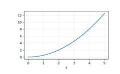
In a second example, we simulate a double integratory''=u, witha constant inputu=1. We’ll use the state space representationof the integrator.

>>>fromscipy.signalimportlti>>>A=np.array([[0.0,1.0],[0.0,0.0]])>>>B=np.array([[0.0],[1.0]])>>>C=np.array([[1.0,0.0]])>>>D=0.0>>>system=lti(A,B,C,D)

t andu define the time and input signal for the system tobe simulated.

>>>t=np.linspace(0,5,num=50)>>>u=np.ones_like(t)

Compute the simulation, and then ploty. As expected, the plot showsthe curvey=0.5*t**2.

>>>tout,y,x=lsim(system,u,t)>>>plt.plot(t,y)>>>plt.grid(alpha=0.3)>>>plt.xlabel('t')>>>plt.show()

Go BackOpen In Tab