freqz#

scipy.signal.freqz(b,a=1,worN=512,whole=False,plot=None,fs=6.283185307179586,include_nyquist=False)[source]#

Compute the frequency response of a digital filter.

Given the M-order numeratorb and N-order denominatora of a digitalfilter, compute its frequency response:

jw-jw-jwMjwB(e)b[0]+b[1]e+...+b[M]eH(e)=------=-----------------------------------jw-jw-jwNA(e)a[0]+a[1]e+...+a[N]e

Parameters:

barray_like

Numerator of a linear filter. Ifb has dimension greater than 1,it is assumed that the coefficients are stored in the first dimension,andb.shape[1:],a.shape[1:], and the shape of the frequenciesarray must be compatible for broadcasting.

aarray_like

Denominator of a linear filter. Ifb has dimension greater than 1,it is assumed that the coefficients are stored in the first dimension,andb.shape[1:],a.shape[1:], and the shape of the frequenciesarray must be compatible for broadcasting.

worN{None, int, array_like}, optional

If a single integer, then compute at that many frequencies (default isN=512). This is a convenient alternative to:

np.linspace(0,fsifwholeelsefs/2,N,endpoint=include_nyquist)

Using a number that is fast for FFT computations can result infaster computations (see Notes).

If an array_like, compute the response at the frequencies given.These are in the same units asfs.

wholebool, optional

Normally, frequencies are computed from 0 to the Nyquist frequency,fs/2 (upper-half of unit-circle). Ifwhole is True, computefrequencies from 0 to fs. Ignored if worN is array_like.

plotcallable

A callable that takes two arguments. If given, the return parametersw andh are passed to plot. Useful for plotting the frequencyresponse insidefreqz.

fsfloat, optional

The sampling frequency of the digital system. Defaults to 2*piradians/sample (so w is from 0 to pi).

Added in version 1.2.0.

include_nyquistbool, optional

Ifwhole is False andworN is an integer, settinginclude_nyquistto True will include the last frequency (Nyquist frequency) and isotherwise ignored.

Added in version 1.5.0.

Returns:

wndarray

The frequencies at whichh was computed, in the same units asfs.By default,w is normalized to the range [0, pi) (radians/sample).

hndarray

The frequency response, as complex numbers.

See also

freqz_zpk

freqz_sos

Notes

Using Matplotlib’smatplotlib.pyplot.plot function as the callableforplot produces unexpected results, as this plots the real part of thecomplex transfer function, not the magnitude.Trylambdaw,h:plot(w,np.abs(h)).

A direct computation via (R)FFT is used to compute the frequency responsewhen the following conditions are met:

1. An integer value is given forworN.

2. worN is fast to compute via FFT (i.e.,next_fast_len(worN) equalsworN).

3. The denominator coefficients are a single value (a.shape[0]==1).

4. worN is at least as long as the numerator coefficients(worN>=b.shape[0]).

5. Ifb.ndim>1, thenb.shape[-1]==1.

For long FIR filters, the FFT approach can have lower error and be muchfaster than the equivalent direct polynomial calculation.

Examples

Try it in your browser!

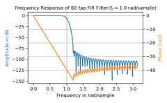
>>>fromscipyimportsignal>>>importnumpyasnp>>>taps,f_c=80,1.0# number of taps and cut-off frequency>>>b=signal.firwin(taps,f_c,window=('kaiser',8),fs=2*np.pi)>>>w,h=signal.freqz(b)

>>>importmatplotlib.pyplotasplt>>>fig,ax1=plt.subplots(tight_layout=True)>>>ax1.set_title(f"Frequency Response of{taps} tap FIR Filter"+...f"($f_c={f_c}$ rad/sample)")>>>ax1.axvline(f_c,color='black',linestyle=':',linewidth=0.8)>>>ax1.plot(w,20*np.log10(abs(h)),'C0')>>>ax1.set_ylabel("Amplitude in dB",color='C0')>>>ax1.set(xlabel="Frequency in rad/sample",xlim=(0,np.pi))

>>>ax2=ax1.twinx()>>>phase=np.unwrap(np.angle(h))>>>ax2.plot(w,phase,'C1')>>>ax2.set_ylabel('Phase [rad]',color='C1')>>>ax2.grid(True)>>>ax2.axis('tight')>>>plt.show()

Broadcasting Examples

Suppose we have two FIR filters whose coefficients are stored in therows of an array with shape (2, 25). For this demonstration, we’lluse random data:

>>>rng=np.random.default_rng()>>>b=rng.random((2,25))

To compute the frequency response for these two filters with one calltofreqz, we must pass inb.T, becausefreqz expects the firstaxis to hold the coefficients. We must then extend the shape with atrivial dimension of length 1 to allow broadcasting with the arrayof frequencies. That is, we pass inb.T[...,np.newaxis], which hasshape (25, 2, 1):

>>>w,h=signal.freqz(b.T[...,np.newaxis],worN=1024)>>>w.shape(1024,)>>>h.shape(2, 1024)

Now, suppose we have two transfer functions, with the same numeratorcoefficientsb=[0.5,0.5]. The coefficients for the two denominatorsare stored in the first dimension of the 2-D arraya:

a=[11][-0.25,-0.5]

>>>b=np.array([0.5,0.5])>>>a=np.array([[1,1],[-0.25,-0.5]])

Onlya is more than 1-D. To make it compatible forbroadcasting with the frequencies, we extend it with a trivial dimensionin the call tofreqz:

>>>w,h=signal.freqz(b,a[...,np.newaxis],worN=1024)>>>w.shape(1024,)>>>h.shape(2, 1024)

Go BackOpen In Tab