Before reading this tutorial you should know a bit of Python. If youwould like to refresh your memory, take a look at thePythontutorial.
If you wish to work the examples in this tutorial, you must also havesome software installed on your computer. Please seehttp://scipy.org/install.html for instructions.
NumPy’s main object is the homogeneous multidimensional array. It is atable of elements (usually numbers), all of the same type, indexed by atuple of positive integers. In NumPy dimensions are calledaxes.
For example, the coordinates of a point in 3D space[1, 2, 1] hasone axis. That axis has 3 elements in it, so we say it has a lengthof 3. In the example pictured below, the array has 2 axes. The firstaxis has a length of 2, the second axis has a length of 3.
[[1.,0.,0.],[0.,1.,2.]]
NumPy’s array class is calledndarray. It is also known by the aliasarray. Note thatnumpy.array is not the same as the StandardPython Library classarray.array, which only handles one-dimensionalarrays and offers less functionality. The more important attributes ofanndarray object are:
shape will be(n,m). The length of theshape tuple is therefore the number of axes,ndim.shape.float64 hasitemsize 8 (=64/8),while one of typecomplex32 hasitemsize 4 (=32/8). It isequivalent tondarray.dtype.itemsize.>>>importnumpyasnp>>>a=np.arange(15).reshape(3,5)>>>aarray([[ 0, 1, 2, 3, 4], [ 5, 6, 7, 8, 9], [10, 11, 12, 13, 14]])>>>a.shape(3, 5)>>>a.ndim2>>>a.dtype.name'int64'>>>a.itemsize8>>>a.size15>>>type(a)<type 'numpy.ndarray'>>>>b=np.array([6,7,8])>>>barray([6, 7, 8])>>>type(b)<type 'numpy.ndarray'>
There are several ways to create arrays.
For example, you can create an array from a regular Python list or tupleusing thearray function. The type of the resulting array is deducedfrom the type of the elements in the sequences.
>>>importnumpyasnp>>>a=np.array([2,3,4])>>>aarray([2, 3, 4])>>>a.dtypedtype('int64')>>>b=np.array([1.2,3.5,5.1])>>>b.dtypedtype('float64')
A frequent error consists in callingarray with multiple numericarguments, rather than providing a single list of numbers as anargument.
>>>a=np.array(1,2,3,4)# WRONG>>>a=np.array([1,2,3,4])# RIGHT
array transforms sequences of sequences into two-dimensional arrays,sequences of sequences of sequences into three-dimensional arrays, andso on.
>>>b=np.array([(1.5,2,3),(4,5,6)])>>>barray([[ 1.5, 2. , 3. ], [ 4. , 5. , 6. ]])
The type of the array can also be explicitly specified at creation time:
>>>c=np.array([[1,2],[3,4]],dtype=complex)>>>carray([[ 1.+0.j, 2.+0.j], [ 3.+0.j, 4.+0.j]])
Often, the elements of an array are originally unknown, but its size isknown. Hence, NumPy offers several functions to createarrays with initial placeholder content. These minimize the necessity ofgrowing arrays, an expensive operation.
The functionzeros creates an array full of zeros, the functionones creates an array full of ones, and the functionemptycreates an array whose initial content is random and depends on thestate of the memory. By default, the dtype of the created array isfloat64.
>>>np.zeros((3,4))array([[ 0., 0., 0., 0.], [ 0., 0., 0., 0.], [ 0., 0., 0., 0.]])>>>np.ones((2,3,4),dtype=np.int16)# dtype can also be specifiedarray([[[ 1, 1, 1, 1], [ 1, 1, 1, 1], [ 1, 1, 1, 1]], [[ 1, 1, 1, 1], [ 1, 1, 1, 1], [ 1, 1, 1, 1]]], dtype=int16)>>>np.empty((2,3))# uninitialized, output may varyarray([[ 3.73603959e-262, 6.02658058e-154, 6.55490914e-260], [ 5.30498948e-313, 3.14673309e-307, 1.00000000e+000]])
To create sequences of numbers, NumPy provides a function analogous torange that returns arrays instead of lists.
>>>np.arange(10,30,5)array([10, 15, 20, 25])>>>np.arange(0,2,0.3)# it accepts float argumentsarray([ 0. , 0.3, 0.6, 0.9, 1.2, 1.5, 1.8])
Whenarange is used with floating point arguments, it is generallynot possible to predict the number of elements obtained, due to thefinite floating point precision. For this reason, it is usually betterto use the functionlinspace that receives as an argument the numberof elements that we want, instead of the step:
>>>fromnumpyimportpi>>>np.linspace(0,2,9)# 9 numbers from 0 to 2array([ 0. , 0.25, 0.5 , 0.75, 1. , 1.25, 1.5 , 1.75, 2. ])>>>x=np.linspace(0,2*pi,100)# useful to evaluate function at lots of points>>>f=np.sin(x)
When you print an array, NumPy displays it in a similar way to nestedlists, but with the following layout:
One-dimensional arrays are then printed as rows, bidimensionals asmatrices and tridimensionals as lists of matrices.
>>>a=np.arange(6)# 1d array>>>print(a)[0 1 2 3 4 5]>>>>>>b=np.arange(12).reshape(4,3)# 2d array>>>print(b)[[ 0 1 2] [ 3 4 5] [ 6 7 8] [ 9 10 11]]>>>>>>c=np.arange(24).reshape(2,3,4)# 3d array>>>print(c)[[[ 0 1 2 3] [ 4 5 6 7] [ 8 9 10 11]] [[12 13 14 15] [16 17 18 19] [20 21 22 23]]]
Seebelow to getmore details onreshape.
If an array is too large to be printed, NumPy automatically skips thecentral part of the array and only prints the corners:
>>>print(np.arange(10000))[ 0 1 2 ..., 9997 9998 9999]>>>>>>print(np.arange(10000).reshape(100,100))[[ 0 1 2 ..., 97 98 99] [ 100 101 102 ..., 197 198 199] [ 200 201 202 ..., 297 298 299] ..., [9700 9701 9702 ..., 9797 9798 9799] [9800 9801 9802 ..., 9897 9898 9899] [9900 9901 9902 ..., 9997 9998 9999]]
To disable this behaviour and force NumPy to print the entire array, youcan change the printing options usingset_printoptions.
>>>np.set_printoptions(threshold=np.nan)
Arithmetic operators on arrays applyelementwise. A new array iscreated and filled with the result.
>>>a=np.array([20,30,40,50])>>>b=np.arange(4)>>>barray([0, 1, 2, 3])>>>c=a-b>>>carray([20, 29, 38, 47])>>>b**2array([0, 1, 4, 9])>>>10*np.sin(a)array([ 9.12945251, -9.88031624, 7.4511316 , -2.62374854])>>>a<35array([ True, True, False, False])
Unlike in many matrix languages, the product operator* operateselementwise in NumPy arrays. The matrix product can be performed usingthe@ operator (in python >=3.5) or thedot function or method:
>>>A=np.array([[1,1],...[0,1]])>>>B=np.array([[2,0],...[3,4]])>>>A*B# elementwise productarray([[2, 0], [0, 4]])>>>A@B# matrix productarray([[5, 4], [3, 4]])>>>A.dot(B)# another matrix productarray([[5, 4], [3, 4]])
Some operations, such as+= and*=, act in place to modify anexisting array rather than create a new one.
>>>a=np.ones((2,3),dtype=int)>>>b=np.random.random((2,3))>>>a*=3>>>aarray([[3, 3, 3], [3, 3, 3]])>>>b+=a>>>barray([[ 3.417022 , 3.72032449, 3.00011437], [ 3.30233257, 3.14675589, 3.09233859]])>>>a+=b# b is not automatically converted to integer typeTraceback (most recent call last):...TypeError:Cannot cast ufunc add output from dtype('float64') to dtype('int64') with casting rule 'same_kind'
When operating with arrays of different types, the type of the resultingarray corresponds to the more general or precise one (a behavior knownas upcasting).
>>>a=np.ones(3,dtype=np.int32)>>>b=np.linspace(0,pi,3)>>>b.dtype.name'float64'>>>c=a+b>>>carray([ 1. , 2.57079633, 4.14159265])>>>c.dtype.name'float64'>>>d=np.exp(c*1j)>>>darray([ 0.54030231+0.84147098j, -0.84147098+0.54030231j, -0.54030231-0.84147098j])>>>d.dtype.name'complex128'
Many unary operations, such as computing the sum of all the elements inthe array, are implemented as methods of thendarray class.
>>>a=np.random.random((2,3))>>>aarray([[ 0.18626021, 0.34556073, 0.39676747], [ 0.53881673, 0.41919451, 0.6852195 ]])>>>a.sum()2.5718191614547998>>>a.min()0.1862602113776709>>>a.max()0.6852195003967595
By default, these operations apply to the array as though it were a listof numbers, regardless of its shape. However, by specifying theaxisparameter you can apply an operation along the specified axis of anarray:
>>>b=np.arange(12).reshape(3,4)>>>barray([[ 0, 1, 2, 3], [ 4, 5, 6, 7], [ 8, 9, 10, 11]])>>>>>>b.sum(axis=0)# sum of each columnarray([12, 15, 18, 21])>>>>>>b.min(axis=1)# min of each rowarray([0, 4, 8])>>>>>>b.cumsum(axis=1)# cumulative sum along each rowarray([[ 0, 1, 3, 6], [ 4, 9, 15, 22], [ 8, 17, 27, 38]])
NumPy provides familiar mathematical functions such as sin, cos, andexp. In NumPy, these are called “universalfunctions”(ufunc). Within NumPy, these functionsoperate elementwise on an array, producing an array as output.
>>>B=np.arange(3)>>>Barray([0, 1, 2])>>>np.exp(B)array([ 1. , 2.71828183, 7.3890561 ])>>>np.sqrt(B)array([ 0. , 1. , 1.41421356])>>>C=np.array([2.,-1.,4.])>>>np.add(B,C)array([ 2., 0., 6.])
One-dimensional arrays can be indexed, sliced and iterated over,much likelistsand other Python sequences.
>>>a=np.arange(10)**3>>>aarray([ 0, 1, 8, 27, 64, 125, 216, 343, 512, 729])>>>a[2]8>>>a[2:5]array([ 8, 27, 64])>>>a[:6:2]=-1000# equivalent to a[0:6:2] = -1000; from start to position 6, exclusive, set every 2nd element to -1000>>>aarray([-1000, 1, -1000, 27, -1000, 125, 216, 343, 512, 729])>>>a[::-1]# reversed aarray([ 729, 512, 343, 216, 125, -1000, 27, -1000, 1, -1000])>>>foriina:...print(i**(1/3.))...nan1.0nan3.0nan5.06.07.08.09.0
Multidimensional arrays can have one index per axis. These indicesare given in a tuple separated by commas:
>>>deff(x,y):...return10*x+y...>>>b=np.fromfunction(f,(5,4),dtype=int)>>>barray([[ 0, 1, 2, 3], [10, 11, 12, 13], [20, 21, 22, 23], [30, 31, 32, 33], [40, 41, 42, 43]])>>>b[2,3]23>>>b[0:5,1]# each row in the second column of barray([ 1, 11, 21, 31, 41])>>>b[:,1]# equivalent to the previous examplearray([ 1, 11, 21, 31, 41])>>>b[1:3,:]# each column in the second and third row of barray([[10, 11, 12, 13], [20, 21, 22, 23]])
When fewer indices are provided than the number of axes, the missingindices are considered complete slices:
>>>b[-1]# the last row. Equivalent to b[-1,:]array([40, 41, 42, 43])
The expression within brackets inb[i] is treated as anifollowed by as many instances of: as needed to represent theremaining axes. NumPy also allows you to write this using dots asb[i,...].
Thedots (...) represent as many colons as needed to produce acomplete indexing tuple. For example, ifx is an array with 5axes, then
x[1,2,...] is equivalent tox[1,2,:,:,:],x[...,3] tox[:,:,:,:,3] andx[4,...,5,:] tox[4,:,:,5,:].>>>c=np.array([[[0,1,2],# a 3D array (two stacked 2D arrays)...[10,12,13]],...[[100,101,102],...[110,112,113]]])>>>c.shape(2, 2, 3)>>>c[1,...]# same as c[1,:,:] or c[1]array([[100, 101, 102], [110, 112, 113]])>>>c[...,2]# same as c[:,:,2]array([[ 2, 13], [102, 113]])
Iterating over multidimensional arrays is done with respect to thefirst axis:
>>>forrowinb:...print(row)...[0 1 2 3][10 11 12 13][20 21 22 23][30 31 32 33][40 41 42 43]
However, if one wants to perform an operation on each element in thearray, one can use theflat attribute which is aniteratorover all the elements of the array:
>>>forelementinb.flat:...print(element)...012310111213202122233031323340414243
See also
Indexing,Indexing (reference),newaxis,ndenumerate,indices
An array has a shape given by the number of elements along each axis:
>>>a=np.floor(10*np.random.random((3,4)))>>>aarray([[ 2., 8., 0., 6.], [ 4., 5., 1., 1.], [ 8., 9., 3., 6.]])>>>a.shape(3, 4)
The shape of an array can be changed with various commands. Note that thefollowing three commands all return a modified array, but do not changethe original array:
>>>a.ravel()# returns the array, flattenedarray([ 2., 8., 0., 6., 4., 5., 1., 1., 8., 9., 3., 6.])>>>a.reshape(6,2)# returns the array with a modified shapearray([[ 2., 8.], [ 0., 6.], [ 4., 5.], [ 1., 1.], [ 8., 9.], [ 3., 6.]])>>>a.T# returns the array, transposedarray([[ 2., 4., 8.], [ 8., 5., 9.], [ 0., 1., 3.], [ 6., 1., 6.]])>>>a.T.shape(4, 3)>>>a.shape(3, 4)
The order of the elements in the array resulting from ravel() isnormally “C-style”, that is, the rightmost index “changes the fastest”,so the element after a[0,0] is a[0,1]. If the array is reshaped to someother shape, again the array is treated as “C-style”. NumPy normallycreates arrays stored in this order, so ravel() will usually not need tocopy its argument, but if the array was made by taking slices of anotherarray or created with unusual options, it may need to be copied. Thefunctions ravel() and reshape() can also be instructed, using anoptional argument, to use FORTRAN-style arrays, in which the leftmostindex changes the fastest.
Thereshape function returns itsargument with a modified shape, whereas thendarray.resize method modifies the arrayitself:
>>>aarray([[ 2., 8., 0., 6.], [ 4., 5., 1., 1.], [ 8., 9., 3., 6.]])>>>a.resize((2,6))>>>aarray([[ 2., 8., 0., 6., 4., 5.], [ 1., 1., 8., 9., 3., 6.]])
If a dimension is given as -1 in a reshaping operation, the otherdimensions are automatically calculated:
>>>a.reshape(3,-1)array([[ 2., 8., 0., 6.], [ 4., 5., 1., 1.], [ 8., 9., 3., 6.]])
See also
Several arrays can be stacked together along different axes:
>>>a=np.floor(10*np.random.random((2,2)))>>>aarray([[ 8., 8.], [ 0., 0.]])>>>b=np.floor(10*np.random.random((2,2)))>>>barray([[ 1., 8.], [ 0., 4.]])>>>np.vstack((a,b))array([[ 8., 8.], [ 0., 0.], [ 1., 8.], [ 0., 4.]])>>>np.hstack((a,b))array([[ 8., 8., 1., 8.], [ 0., 0., 0., 4.]])
The functioncolumn_stackstacks 1D arrays as columns into a 2D array. It is equivalent tohstack only for 2D arrays:
>>>fromnumpyimportnewaxis>>>np.column_stack((a,b))# with 2D arraysarray([[ 8., 8., 1., 8.], [ 0., 0., 0., 4.]])>>>a=np.array([4.,2.])>>>b=np.array([3.,8.])>>>np.column_stack((a,b))# returns a 2D arrayarray([[ 4., 3.], [ 2., 8.]])>>>np.hstack((a,b))# the result is differentarray([ 4., 2., 3., 8.])>>>a[:,newaxis]# this allows to have a 2D columns vectorarray([[ 4.], [ 2.]])>>>np.column_stack((a[:,newaxis],b[:,newaxis]))array([[ 4., 3.], [ 2., 8.]])>>>np.hstack((a[:,newaxis],b[:,newaxis]))# the result is the samearray([[ 4., 3.], [ 2., 8.]])
On the other hand, the functionrow_stack is equivalent tovstackfor any input arrays.In general, for arrays of with more than two dimensions,hstack stacks along their secondaxes,vstack stacks along theirfirst axes, andconcatenateallows for an optional arguments giving the number of the axis alongwhich the concatenation should happen.
Note
In complex cases,r_ andc_ are useful for creating arraysby stacking numbers along one axis. They allow the use of range literals(“:”)
>>>np.r_[1:4,0,4]array([1, 2, 3, 0, 4])
When used with arrays as arguments,r_ andc_ are similar tovstack andhstack in their default behavior,but allow for an optional argument giving the number of the axis alongwhich to concatenate.
See also
Usinghsplit, you can split anarray along its horizontal axis, either by specifying the number ofequally shaped arrays to return, or by specifying the columns afterwhich the division should occur:
>>>a=np.floor(10*np.random.random((2,12)))>>>aarray([[ 9., 5., 6., 3., 6., 8., 0., 7., 9., 7., 2., 7.], [ 1., 4., 9., 2., 2., 1., 0., 6., 2., 2., 4., 0.]])>>>np.hsplit(a,3)# Split a into 3[array([[ 9., 5., 6., 3.], [ 1., 4., 9., 2.]]), array([[ 6., 8., 0., 7.], [ 2., 1., 0., 6.]]), array([[ 9., 7., 2., 7.], [ 2., 2., 4., 0.]])]>>>np.hsplit(a,(3,4))# Split a after the third and the fourth column[array([[ 9., 5., 6.], [ 1., 4., 9.]]), array([[ 3.], [ 2.]]), array([[ 6., 8., 0., 7., 9., 7., 2., 7.], [ 2., 1., 0., 6., 2., 2., 4., 0.]])]
vsplit splits along the verticalaxis, andarray_split allowsone to specify along which axis to split.
When operating and manipulating arrays, their data is sometimes copiedinto a new array and sometimes not. This is often a source of confusionfor beginners. There are three cases:
Simple assignments make no copy of array objects or of their data.
>>>a=np.arange(12)>>>b=a# no new object is created>>>bisa# a and b are two names for the same ndarray objectTrue>>>b.shape=3,4# changes the shape of a>>>a.shape(3, 4)
Python passes mutable objects as references, so function calls make nocopy.
>>>deff(x):...print(id(x))...>>>id(a)# id is a unique identifier of an object148293216>>>f(a)148293216
Different array objects can share the same data. Theview methodcreates a new array object that looks at the same data.
>>>c=a.view()>>>cisaFalse>>>c.baseisa# c is a view of the data owned by aTrue>>>c.flags.owndataFalse>>>>>>c.shape=2,6# a's shape doesn't change>>>a.shape(3, 4)>>>c[0,4]=1234# a's data changes>>>aarray([[ 0, 1, 2, 3], [1234, 5, 6, 7], [ 8, 9, 10, 11]])
Slicing an array returns a view of it:
>>>s=a[:,1:3]# spaces added for clarity; could also be written "s = a[:,1:3]">>>s[:]=10# s[:] is a view of s. Note the difference between s=10 and s[:]=10>>>aarray([[ 0, 10, 10, 3], [1234, 10, 10, 7], [ 8, 10, 10, 11]])
Thecopy method makes a complete copy of the array and its data.
>>>d=a.copy()# a new array object with new data is created>>>disaFalse>>>d.baseisa# d doesn't share anything with aFalse>>>d[0,0]=9999>>>aarray([[ 0, 10, 10, 3], [1234, 10, 10, 7], [ 8, 10, 10, 11]])
Here is a list of some useful NumPy functions and methods namesordered in categories. SeeRoutines for the full list.
arange,array,copy,empty,empty_like,eye,fromfile,fromfunction,identity,linspace,logspace,mgrid,ogrid,ones,ones_like,r,zeros,zeros_likendarray.astype,atleast_1d,atleast_2d,atleast_3d,matarray_split,column_stack,concatenate,diagonal,dsplit,dstack,hsplit,hstack,ndarray.item,newaxis,ravel,repeat,reshape,resize,squeeze,swapaxes,take,transpose,vsplit,vstackall,any,nonzero,whereargmax,argmin,argsort,max,min,ptp,searchsorted,sortchoose,compress,cumprod,cumsum,inner,ndarray.fill,imag,prod,put,putmask,real,sumcov,mean,std,varcross,dot,outer,linalg.svd,vdotBroadcasting allows universal functions to deal in a meaningful way withinputs that do not have exactly the same shape.
The first rule of broadcasting is that if all input arrays do not havethe same number of dimensions, a “1” will be repeatedly prepended to theshapes of the smaller arrays until all the arrays have the same numberof dimensions.
The second rule of broadcasting ensures that arrays with a size of 1along a particular dimension act as if they had the size of the arraywith the largest shape along that dimension. The value of the arrayelement is assumed to be the same along that dimension for the“broadcast” array.
After application of the broadcasting rules, the sizes of all arraysmust match. More details can be found inBroadcasting.
NumPy offers more indexing facilities than regular Python sequences. Inaddition to indexing by integers and slices, as we saw before, arrayscan be indexed by arrays of integers and arrays of booleans.
>>>a=np.arange(12)**2# the first 12 square numbers>>>i=np.array([1,1,3,8,5])# an array of indices>>>a[i]# the elements of a at the positions iarray([ 1, 1, 9, 64, 25])>>>>>>j=np.array([[3,4],[9,7]])# a bidimensional array of indices>>>a[j]# the same shape as jarray([[ 9, 16], [81, 49]])
When the indexed arraya is multidimensional, a single array ofindices refers to the first dimension ofa. The following exampleshows this behavior by converting an image of labels into a color imageusing a palette.
>>>palette=np.array([[0,0,0],# black...[255,0,0],# red...[0,255,0],# green...[0,0,255],# blue...[255,255,255]])# white>>>image=np.array([[0,1,2,0],# each value corresponds to a color in the palette...[0,3,4,0]])>>>palette[image]# the (2,4,3) color imagearray([[[ 0, 0, 0], [255, 0, 0], [ 0, 255, 0], [ 0, 0, 0]], [[ 0, 0, 0], [ 0, 0, 255], [255, 255, 255], [ 0, 0, 0]]])
We can also give indexes for more than one dimension. The arrays ofindices for each dimension must have the same shape.
>>>a=np.arange(12).reshape(3,4)>>>aarray([[ 0, 1, 2, 3], [ 4, 5, 6, 7], [ 8, 9, 10, 11]])>>>i=np.array([[0,1],# indices for the first dim of a...[1,2]])>>>j=np.array([[2,1],# indices for the second dim...[3,3]])>>>>>>a[i,j]# i and j must have equal shapearray([[ 2, 5], [ 7, 11]])>>>>>>a[i,2]array([[ 2, 6], [ 6, 10]])>>>>>>a[:,j]# i.e., a[ : , j]array([[[ 2, 1], [ 3, 3]], [[ 6, 5], [ 7, 7]], [[10, 9], [11, 11]]])
Naturally, we can puti andj in a sequence (say a list) andthen do the indexing with the list.
>>>l=[i,j]>>>a[l]# equivalent to a[i,j]array([[ 2, 5], [ 7, 11]])
However, we can not do this by puttingi andj into an array,because this array will be interpreted as indexing the first dimensionof a.
>>>s=np.array([i,j])>>>a[s]# not what we wantTraceback (most recent call last): File"<stdin>", line1, in?IndexError:index (3) out of range (0<=index<=2) in dimension 0>>>>>>a[tuple(s)]# same as a[i,j]array([[ 2, 5], [ 7, 11]])
Another common use of indexing with arrays is the search of the maximumvalue of time-dependent series:
>>>time=np.linspace(20,145,5)# time scale>>>data=np.sin(np.arange(20)).reshape(5,4)# 4 time-dependent series>>>timearray([ 20. , 51.25, 82.5 , 113.75, 145. ])>>>dataarray([[ 0. , 0.84147098, 0.90929743, 0.14112001], [-0.7568025 , -0.95892427, -0.2794155 , 0.6569866 ], [ 0.98935825, 0.41211849, -0.54402111, -0.99999021], [-0.53657292, 0.42016704, 0.99060736, 0.65028784], [-0.28790332, -0.96139749, -0.75098725, 0.14987721]])>>>>>>ind=data.argmax(axis=0)# index of the maxima for each series>>>indarray([2, 0, 3, 1])>>>>>>time_max=time[ind]# times corresponding to the maxima>>>>>>data_max=data[ind,range(data.shape[1])]# => data[ind[0],0], data[ind[1],1]...>>>>>>time_maxarray([ 82.5 , 20. , 113.75, 51.25])>>>data_maxarray([ 0.98935825, 0.84147098, 0.99060736, 0.6569866 ])>>>>>>np.all(data_max==data.max(axis=0))True
You can also use indexing with arrays as a target to assign to:
>>>a=np.arange(5)>>>aarray([0, 1, 2, 3, 4])>>>a[[1,3,4]]=0>>>aarray([0, 0, 2, 0, 0])
However, when the list of indices contains repetitions, the assignmentis done several times, leaving behind the last value:
>>>a=np.arange(5)>>>a[[0,0,2]]=[1,2,3]>>>aarray([2, 1, 3, 3, 4])
This is reasonable enough, but watch out if you want to use Python’s+= construct, as it may not do what you expect:
>>>a=np.arange(5)>>>a[[0,0,2]]+=1>>>aarray([1, 1, 3, 3, 4])
Even though 0 occurs twice in the list of indices, the 0th element isonly incremented once. This is because Python requires “a+=1” to beequivalent to “a = a + 1”.
When we index arrays with arrays of (integer) indices we are providingthe list of indices to pick. With boolean indices the approach isdifferent; we explicitly choose which items in the array we want andwhich ones we don’t.
The most natural way one can think of for boolean indexing is to useboolean arrays that havethe same shape as the original array:
>>>a=np.arange(12).reshape(3,4)>>>b=a>4>>>b# b is a boolean with a's shapearray([[False, False, False, False], [False, True, True, True], [ True, True, True, True]])>>>a[b]# 1d array with the selected elementsarray([ 5, 6, 7, 8, 9, 10, 11])
This property can be very useful in assignments:
>>>a[b]=0# All elements of 'a' higher than 4 become 0>>>aarray([[0, 1, 2, 3], [4, 0, 0, 0], [0, 0, 0, 0]])
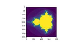
You can look at the followingexample to seehow to use boolean indexing to generate an image of theMandelbrotset:
>>>importnumpyasnp>>>importmatplotlib.pyplotasplt>>>defmandelbrot(h,w,maxit=20):..."""Returns an image of the Mandelbrot fractal of size (h,w)."""...y,x=np.ogrid[-1.4:1.4:h*1j,-2:0.8:w*1j]...c=x+y*1j...z=c...divtime=maxit+np.zeros(z.shape,dtype=int)......foriinrange(maxit):...z=z**2+c...diverge=z*np.conj(z)>2**2# who is diverging...div_now=diverge&(divtime==maxit)# who is diverging now...divtime[div_now]=i# note when...z[diverge]=2# avoid diverging too much......returndivtime>>>plt.imshow(mandelbrot(400,400))>>>plt.show()
The second way of indexing with booleans is more similar to integerindexing; for each dimension of the array we give a 1D boolean arrayselecting the slices we want:
>>>a=np.arange(12).reshape(3,4)>>>b1=np.array([False,True,True])# first dim selection>>>b2=np.array([True,False,True,False])# second dim selection>>>>>>a[b1,:]# selecting rowsarray([[ 4, 5, 6, 7], [ 8, 9, 10, 11]])>>>>>>a[b1]# same thingarray([[ 4, 5, 6, 7], [ 8, 9, 10, 11]])>>>>>>a[:,b2]# selecting columnsarray([[ 0, 2], [ 4, 6], [ 8, 10]])>>>>>>a[b1,b2]# a weird thing to doarray([ 4, 10])
Note that the length of the 1D boolean array must coincide with thelength of the dimension (or axis) you want to slice. In the previousexample,b1 has length 3 (the number ofrows ina), andb2 (of length 4) is suitable to index the 2nd axis (columns) ofa.
Theix_ function can be used to combine different vectors so as toobtain the result for each n-uplet. For example, if you want to computeall the a+b*c for all the triplets taken from each of the vectors a, band c:
>>>a=np.array([2,3,4,5])>>>b=np.array([8,5,4])>>>c=np.array([5,4,6,8,3])>>>ax,bx,cx=np.ix_(a,b,c)>>>axarray([[[2]], [[3]], [[4]], [[5]]])>>>bxarray([[[8], [5], [4]]])>>>cxarray([[[5, 4, 6, 8, 3]]])>>>ax.shape,bx.shape,cx.shape((4, 1, 1), (1, 3, 1), (1, 1, 5))>>>result=ax+bx*cx>>>resultarray([[[42, 34, 50, 66, 26], [27, 22, 32, 42, 17], [22, 18, 26, 34, 14]], [[43, 35, 51, 67, 27], [28, 23, 33, 43, 18], [23, 19, 27, 35, 15]], [[44, 36, 52, 68, 28], [29, 24, 34, 44, 19], [24, 20, 28, 36, 16]], [[45, 37, 53, 69, 29], [30, 25, 35, 45, 20], [25, 21, 29, 37, 17]]])>>>result[3,2,4]17>>>a[3]+b[2]*c[4]17
You could also implement the reduce as follows:
>>>defufunc_reduce(ufct,*vectors):...vs=np.ix_(*vectors)...r=ufct.identity...forvinvs:...r=ufct(r,v)...returnr
and then use it as:
>>>ufunc_reduce(np.add,a,b,c)array([[[15, 14, 16, 18, 13], [12, 11, 13, 15, 10], [11, 10, 12, 14, 9]], [[16, 15, 17, 19, 14], [13, 12, 14, 16, 11], [12, 11, 13, 15, 10]], [[17, 16, 18, 20, 15], [14, 13, 15, 17, 12], [13, 12, 14, 16, 11]], [[18, 17, 19, 21, 16], [15, 14, 16, 18, 13], [14, 13, 15, 17, 12]]])
The advantage of this version of reduce compared to the normalufunc.reduce is that it makes use of theBroadcastingRulesin order to avoid creating an argument array the size of the outputtimes the number of vectors.
Work in progress. Basic linear algebra to be included here.
See linalg.py in numpy folder for more.
>>>importnumpyasnp>>>a=np.array([[1.0,2.0],[3.0,4.0]])>>>print(a)[[ 1. 2.] [ 3. 4.]]>>>a.transpose()array([[ 1., 3.], [ 2., 4.]])>>>np.linalg.inv(a)array([[-2. , 1. ], [ 1.5, -0.5]])>>>u=np.eye(2)# unit 2x2 matrix; "eye" represents "I">>>uarray([[ 1., 0.], [ 0., 1.]])>>>j=np.array([[0.0,-1.0],[1.0,0.0]])>>>j@j# matrix productarray([[-1., 0.], [ 0., -1.]])>>>np.trace(u)# trace2.0>>>y=np.array([[5.],[7.]])>>>np.linalg.solve(a,y)array([[-3.], [ 4.]])>>>np.linalg.eig(j)(array([ 0.+1.j, 0.-1.j]), array([[ 0.70710678+0.j , 0.70710678-0.j ], [ 0.00000000-0.70710678j, 0.00000000+0.70710678j]]))
Parameters: square matrixReturns The eigenvalues, each repeated according to its multiplicity. The normalized (unit "length") eigenvectors, such that the column ``v[:,i]`` is the eigenvector corresponding to the eigenvalue ``w[i]`` .
Here we give a list of short and useful tips.
To change the dimensions of an array, you can omit one of the sizeswhich will then be deduced automatically:
>>>a=np.arange(30)>>>a.shape=2,-1,3# -1 means "whatever is needed">>>a.shape(2, 5, 3)>>>aarray([[[ 0, 1, 2], [ 3, 4, 5], [ 6, 7, 8], [ 9, 10, 11], [12, 13, 14]], [[15, 16, 17], [18, 19, 20], [21, 22, 23], [24, 25, 26], [27, 28, 29]]])
How do we construct a 2D array from a list of equally-sized row vectors?In MATLAB this is quite easy: ifx andy are two vectors of thesame length you only need dom=[x;y]. In NumPy this works via thefunctionscolumn_stack,dstack,hstack andvstack,depending on the dimension in which the stacking is to be done. Forexample:
x=np.arange(0,10,2)# x=([0,2,4,6,8])y=np.arange(5)# y=([0,1,2,3,4])m=np.vstack([x,y])# m=([[0,2,4,6,8],# [0,1,2,3,4]])xy=np.hstack([x,y])# xy =([0,2,4,6,8,0,1,2,3,4])
The logic behind those functions in more than two dimensions can bestrange.
See also
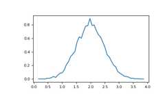
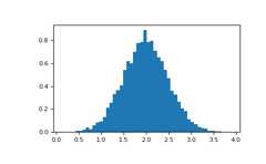
The NumPyhistogram function applied to an array returns a pair ofvectors: the histogram of the array and the vector of bins. Beware:matplotlib also has a function to build histograms (calledhist,as in Matlab) that differs from the one in NumPy. The main difference isthatpylab.hist plots the histogram automatically, whilenumpy.histogram only generates the data.
>>>importnumpyasnp>>>importmatplotlib.pyplotasplt>>># Build a vector of 10000 normal deviates with variance 0.5^2 and mean 2>>>mu,sigma=2,0.5>>>v=np.random.normal(mu,sigma,10000)>>># Plot a normalized histogram with 50 bins>>>plt.hist(v,bins=50,density=1)# matplotlib version (plot)>>>plt.show()
>>># Compute the histogram with numpy and then plot it>>>(n,bins)=np.histogram(v,bins=50,density=True)# NumPy version (no plot)>>>plt.plot(.5*(bins[1:]+bins[:-1]),n)>>>plt.show()