numpy.random.laplace¶

numpy.random.laplace(loc=0.0,scale=1.0,size=None)¶

Draw samples from the Laplace or double exponential distribution withspecified location (or mean) and scale (decay).

The Laplace distribution is similar to the Gaussian/normal distribution,but is sharper at the peak and has fatter tails. It represents thedifference between two independent, identically distributed exponentialrandom variables.

Parameters:

loc:float or array_like of floats, optional The position,\mu, of the distribution peak. Default is 0. scale:float or array_like of floats, optional \lambda, the exponential decay. Default is 1. size:int or tuple of ints, optional Output shape. If the given shape is, e.g.,(m,n,k), thenm*n*k samples are drawn. If size isNone (default),a single value is returned ifloc andscale are both scalars.Otherwise,np.broadcast(loc,scale).size samples are drawn.

Returns:

out:ndarray or scalar Drawn samples from the parameterized Laplace distribution.

Notes

It has the probability density function

f(x; \mu, \lambda) = \frac{1}{2\lambda}\exp\left(-\frac{|x - \mu|}{\lambda}\right).

The first law of Laplace, from 1774, states that the frequencyof an error can be expressed as an exponential function of theabsolute magnitude of the error, which leads to the Laplacedistribution. For many problems in economics and healthsciences, this distribution seems to model the data betterthan the standard Gaussian distribution.

References

[1]	Abramowitz, M. and Stegun, I. A. (Eds.). “Handbook ofMathematical Functions with Formulas, Graphs, and MathematicalTables, 9th printing,” New York: Dover, 1972.

[2]	Kotz, Samuel, et. al. “The Laplace Distribution andGeneralizations, ” Birkhauser, 2001.

[3]	Weisstein, Eric W. “Laplace Distribution.”From MathWorld–A Wolfram Web Resource.http://mathworld.wolfram.com/LaplaceDistribution.html

[4]	Wikipedia, “Laplace distribution”,http://en.wikipedia.org/wiki/Laplace_distribution

Examples

Draw samples from the distribution

>>>loc,scale=0.,1.>>>s=np.random.laplace(loc,scale,1000)

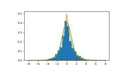
Display the histogram of the samples, along withthe probability density function:

>>>importmatplotlib.pyplotasplt>>>count,bins,ignored=plt.hist(s,30,density=True)>>>x=np.arange(-8.,8.,.01)>>>pdf=np.exp(-abs(x-loc)/scale)/(2.*scale)>>>plt.plot(x,pdf)

Plot Gaussian for comparison:

>>>g=(1/(scale*np.sqrt(2*np.pi))*...np.exp(-(x-loc)**2/(2*scale**2)))>>>plt.plot(x,g)