

Query data in BigQuery from within JupyterLab
This page shows you how to query data that is storedin BigQuery from within the JupyterLab interfaceof your Vertex AI Workbench instance.
Methods for querying BigQuery data in notebook (IPYNB) files
To query BigQuery data from within a JupyterLab notebook file,you can use the%%bigquery magic command andthe BigQuery client library for Python.
Vertex AI Workbench instances alsoinclude a BigQuery integration that lets youbrowse and query data from within the JupyterLab interface.
This page describes how to use each of these methods.
Before you begin
If you haven't already,createa Vertex AI Workbench instance.
Required roles
To ensure that your instance's service account has the necessary permissions to query data in BigQuery, ask your administrator to grant your instance's service account the Service Usage Consumer (roles/serviceusage.serviceUsageConsumer) IAM role on the project.Important: You must grant this role to your instance's service account,not to your user account. Failure to grant the role to the correct principal might result in permission errors. For more information about granting roles, seeManage access to projects, folders, and organizations.
Your administrator might also be able to give your instance's service account the required permissions throughcustom roles or otherpredefined roles.
Open JupyterLab
In the Google Cloud console, go to theInstances page.
Next to your Vertex AI Workbench instance's name,clickOpen JupyterLab.
Your Vertex AI Workbench instance opens JupyterLab.
Browse BigQuery resources
The BigQuery integration provides a pane for browsingthe BigQuery resources that you have access to.
In the JupyterLab navigation menu, click
 BigQuery in Notebooks.
TheBigQuery pane lists available projects and datasets, where youcan perform tasks as follows:
- To view a description of a dataset, double-click the dataset name.
- To show a dataset's tables, views, and models, expand the dataset.
- To open a summary description as a tab in JupyterLab, double-click atable, view, or model.
Note: On the summary description for a table, click thePreviewtab to preview a table's data. The following image shows a preview of the
international_top_termstable found in thegoogle_trendsdataset in thebigquery-public-dataproject: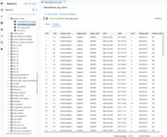
Query data by using the %%bigquery magic command
In this section, you write SQL directly in notebook cells and read data fromBigQuery into the Python notebook.
Magic commands that use a single or double percentage character (% or%%)let you use minimal syntax to interact with BigQuery within thenotebook. The BigQuery client library for Python is automaticallyinstalled in a Vertex AI Workbench instance. Behind the scenes, the%%bigquery magiccommand uses the BigQuery client library for Python to run thegiven query, convert the results to a pandas DataFrame, optionally save theresults to a variable, and then display the results.
Note: As of version 1.26.0 of thegoogle-cloud-bigquery Python package,theBigQuery Storage API is used by default to download results from the%%bigquery magics.
To open a notebook file, selectFile> New>Notebook.
In theSelect Kernel dialog, selectPython 3, and then clickSelect.
Your new IPYNB file opens.
To get the number of regions by country in the
international_top_termsdataset, enter the following statement:%%bigquerySELECTcountry_code,country_name,COUNT(DISTINCTregion_code)ASnum_regionsFROM`bigquery-public-data.google_trends.international_top_terms`WHERErefresh_date=DATE_SUB(CURRENT_DATE,INTERVAL1DAY)GROUPBYcountry_code,country_nameORDERBYnum_regionsDESC;
Click Run cell.
The output is similar to the following:
Query complete after 0.07s: 100%|██████████| 4/4 [00:00<00:00, 1440.60query/s]Downloading: 100%|██████████| 41/41 [00:02<00:00, 20.21rows/s]country_code country_name num_regions0 TR Turkey 811 TH Thailand 772 VN Vietnam 633 JP Japan 474 RO Romania 425 NG Nigeria 376 IN India 367 ID Indonesia 348 CO Colombia 339 MX Mexico 3210 BR Brazil 2711 EG Egypt 2712 UA Ukraine 2713 CH Switzerland 2614 AR Argentina 2415 FR France 2216 SE Sweden 2117 HU Hungary 2018 IT Italy 2019 PT Portugal 2020 NO Norway 1921 FI Finland 1822 NZ New Zealand 1723 PH Philippines 17...
google_trendsdataset being queried is refreshed with new data on an ongoing basis.In the next cell (below the output from the previous cell), enter thefollowing command to run the same query, but this time save the results toa new pandas DataFrame that's named
regions_by_country. You provide thatname by using an argument with the%%bigquerymagic command.%%bigqueryregions_by_countrySELECTcountry_code,country_name,COUNT(DISTINCTregion_code)ASnum_regionsFROM`bigquery-public-data.google_trends.international_top_terms`WHERErefresh_date=DATE_SUB(CURRENT_DATE,INTERVAL1DAY)GROUPBYcountry_code,country_nameORDERBYnum_regionsDESC;
Note: For more information about available arguments for the
%%bigquerycommand, see theclient library magics documentation.Click Run cell.
In the next cell, enter the following command to look at the first fewrows of the query results that you just read in:
regions_by_country.head()Click Run cell.
The pandas DataFrame
regions_by_countryis ready to plot.
Query data by using the BigQuery client library directly
In this section, you use the BigQuery client library for Pythondirectly to read data into the Python notebook.
The client library gives you more control over your queries and lets you usemore complex configurations for queries and jobs. The library's integrationswith pandas enable you to combine the power of declarative SQL with imperativecode (Python) to help you analyze, visualize, and transform your data.
Note: You can use a number of Python data analysis, data wrangling, andvisualization libraries, such asnumpy,pandas,matplotlib, and manyothers. Several of these libraries are built on top of a DataFrame object.
In the next cell, enter the following Python code to import theBigQuery client library for Python and initialize a client:
fromgoogle.cloudimportbigqueryclient=bigquery.Client()The BigQuery client is used to send and receive messagesfrom the BigQuery API.
Click Run cell.
In the next cell, enter the following code to retrieve the percentage ofdaily top terms in the US
top_termsthat overlap across time by number of days apart. The idea here is to lookat each day's top terms and see what percentage of them overlap with thetop terms from the day before, 2 days prior, 3 days prior, and so on (forall pairs of dates over about a month span).sql="""WITH TopTermsByDate AS ( SELECT DISTINCT refresh_date AS date, term FROM `bigquery-public-data.google_trends.top_terms` ), DistinctDates AS ( SELECT DISTINCT date FROM TopTermsByDate )SELECT DATE_DIFF(Dates2.date, Date1Terms.date, DAY) AS days_apart, COUNT(DISTINCT (Dates2.date || Date1Terms.date)) AS num_date_pairs, COUNT(Date1Terms.term) AS num_date1_terms, SUM(IF(Date2Terms.term IS NOT NULL, 1, 0)) AS overlap_terms, SAFE_DIVIDE( SUM(IF(Date2Terms.term IS NOT NULL, 1, 0)), COUNT(Date1Terms.term) ) AS pct_overlap_termsFROM TopTermsByDate AS Date1TermsCROSS JOIN DistinctDates AS Dates2LEFT JOIN TopTermsByDate AS Date2Terms ON Dates2.date = Date2Terms.date AND Date1Terms.term = Date2Terms.termWHERE Date1Terms.date<= Dates2.dateGROUP BY days_apartORDER BY days_apart;"""pct_overlap_terms_by_days_apart=client.query(sql).to_dataframe()pct_overlap_terms_by_days_apart.head()
The SQL being used is encapsulated in a Python string and then passed to the
query()method to run a query. Theto_dataframemethod waits for the query to finish and downloads the results to a pandasDataFrame by using the BigQuery Storage API.Click Runcell.
The first few rows of query results appear below the code cell.
days_apart num_date_pairs num_date1_terms overlap_terms pct_overlap_terms 0 0 32 800 800 1.000000 1 1 31 775 203 0.261935 2 2 30 750 73 0.097333 3 3 29 725 31 0.042759 4 4 28 700 23 0.032857
google_trendsdataset being queried is refreshed with new data on an ongoing basis.
For more information about using BigQuery client libraries, seethe quickstartUsing client libraries.
Query data by using the BigQuery integration in Vertex AI Workbench
The BigQuery integration provides two additional methodsfor querying data. These methods are different from usingthe%%bigquery magic command.
TheIn-cell query editor is a cell type that you can use withinyour notebook files.
TheStand-alone query editor opens as a separate tab in JupyterLab.
In-cell
To use the in-cell query editor to query datain a BigQuery table, complete the following steps:
In JupyterLab, open a notebook (IPYNB) file orcreate a newone.
To create an in-cell query editor, click the cell,and then to the right of the cell, click the BigQuery Integration button.Or in a markdown cell, enter
#@BigQuery.The BigQuery integration converts the cell intoan in-cell query editor.
On a new line below
#@BigQuery, write your query usingthesupported statements and SQL dialects ofBigQuery.If errors are detected in your query, an error message appearsin the top right corner of the query editor. If the query is valid,the estimated number of bytes to be processed appears.ClickSubmit Query. Your query results appear.By default, query results are paginated at 100 rows per pageand limited to 1,000 rows total, but you can changethese settings at the bottom of the results table. In thequery editor, keep the query limited to only the data you needto verify your query. You'll run this query again in a notebook cell,where you can adjust the limit to retrieve thefull results set if you want.
Note: Query text and results persist after closing and reopeningthe notebook file.You can clickQuery and load as DataFrame to automaticallyadd a new cell that contains a code segmentthat imports the BigQuery client library for Python,runs your query in a notebook cell, and stores the resultsin a pandas dataframe named
df.
Stand-alone
To use the stand-alone query editor to query datain a BigQuery table, complete the following steps:
In JupyterLab, in theBigQuery in Notebooks pane, right-clicka table, and selectQuery table,or double-click a table to open a descriptionin a separate tab, and then click theQuery table link.
Write your query using thesupported statements and SQL dialects ofBigQuery.If errors are detected in your query, an error message appearsin the top right corner of the query editor. If the query is valid,the estimated number of bytes to be processed appears.
ClickSubmit Query. Your query results appear.By default, query results are paginated at 100 rows per pageand limited to 1,000 rows total, but you can changethese settings at the bottom of the results table. In thequery editor, keep the query limited to only the data you needto verify your query. You'll run this query again in a notebook cell,where you can adjust the limit to retrieve thefull results set if you want.
You can clickCopy code for DataFrame to copy a code segmentthat imports the BigQuery client library for Python,runs your query in a notebook cell, and stores the resultsin a pandas dataframe named
df. Paste this code into a notebook cellwhere you want to run it.
View query history and reuse queries
To view your query history as a tab in JupyterLab, perform the following steps:
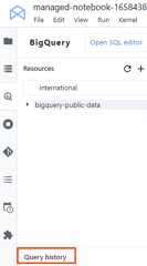
In the JupyterLab navigation menu, click
BigQuery in Notebooks to open theBigQuery pane.In theBigQuery pane, scroll down and clickQuery history.
A list of your queries opens in a new tab, where you can perform tasks suchas the following:
- To view the details of a query such as its Job ID, when the query wasrun, and how long it took, click the query.
- To revise the query, run it again, or copy it into your notebook forfuture use, clickOpen query in editor.
What's next
To see examples of how to visualize the data fromyour BigQuery tables, seeExplore and visualize datain BigQuery fromwithin JupyterLab.
To learn more about writing queries for BigQuery, seeRunning interactive and batch query jobs.
Learn how tocontrol access toBigQuery datasets.
Learn how toaccess Cloud Storage buckets and filesfrom within JupyterLab.
Except as otherwise noted, the content of this page is licensed under theCreative Commons Attribution 4.0 License, and code samples are licensed under theApache 2.0 License. For details, see theGoogle Developers Site Policies. Java is a registered trademark of Oracle and/or its affiliates.
Last updated 2025-12-15 UTC.