Create a dataset

Create a BigQuery dataset to store your ML model.

{"datasetReference":{"datasetId":"bqml_tutorial"}}

importgoogle.cloud.bigquerybqclient=google.cloud.bigquery.Client()bqclient.create_dataset("bqml_tutorial",exists_ok=True)

Create a table of input data

Create a table of data that you can use to train and evaluate the model. Thistable combines columns from several tables in thebigquery-public-data.epa_historical_air_quality dataset in order to providedaily data weather data. You also create the following columns to use asinput variables for the model:

• date: the date of the observation
• pm25 the average PM2.5 value for each day
• wind_speed: the average wind speed for each day
• temperature: the highest temperature for each day

In the following GoogleSQL query, theFROM bigquery-public-data.epa_historical_air_quality.*_daily_summary clauseindicates that you are querying the*_daily_summary tables in theepa_historical_air_quality dataset. These tables arepartitioned tables.

Follow these steps to create the input data table:

1. In the Google Cloud console, go to theBigQuery page.

   Go to BigQuery

2. In the query editor, paste in the following query and clickRun:

   CREATETABLE`bqml_tutorial.seattle_air_quality_daily`ASWITHpm25_dailyAS(SELECTavg(arithmetic_mean)ASpm25,date_localASdateFROM`bigquery-public-data.epa_historical_air_quality.pm25_nonfrm_daily_summary`WHEREcity_name='Seattle'ANDparameter_name='Acceptable PM2.5 AQI & Speciation Mass'GROUPBYdate_local),wind_speed_dailyAS(SELECTavg(arithmetic_mean)ASwind_speed,date_localASdateFROM`bigquery-public-data.epa_historical_air_quality.wind_daily_summary`WHEREcity_name='Seattle'ANDparameter_name='Wind Speed - Resultant'GROUPBYdate_local),temperature_dailyAS(SELECTavg(first_max_value)AStemperature,date_localASdateFROM`bigquery-public-data.epa_historical_air_quality.temperature_daily_summary`WHEREcity_name='Seattle'ANDparameter_name='Outdoor Temperature'GROUPBYdate_local)SELECTpm25_daily.dateASdate,pm25,wind_speed,temperatureFROMpm25_dailyJOINwind_speed_dailyUSING(date)JOINtemperature_dailyUSING(date);

Visualize the input data

Before creating the model, you can optionally visualize your inputtime series data to get a sense of the distribution. You can do this by usingLooker Studio.

Follow these steps to visualize the time series data:

1. In the Google Cloud console, go to theBigQuery page.

   Go to BigQuery

2. In the query editor, paste in the following query and clickRun:

   SELECT*FROM`bqml_tutorial.seattle_air_quality_daily`;

3. When the query completes, clickOpen in>Looker Studio. Looker Studio opens ina new tab. Complete the following steps in the new tab.

4. In the Looker Studio, clickInsert>Time series chart.

5. In theChart pane, choose theSetup tab.

6. In theMetric section, add thepm25,temperature, andwind_speed fields, and remove the defaultRecord Count metric.The resulting chart looks similar to the following:

   

   Looking at the chart, you can see that the input time series has a weeklyseasonal pattern.

Create the time series model

Create a time series model to forecast particulate matter values, as representedby thepm25 column, using thepm25,wind_speed, andtemperature columnvalues as input variables. Train the model on the air quality data from thebqml_tutorial.seattle_air_quality_daily table, selecting the data gatheredbetween January 1, 2012 and December 31, 2020.

In the following query, theOPTIONS(model_type='ARIMA_PLUS_XREG',time_series_timestamp_col='date', ...) clause indicates that you are creatingan ARIMA with external regressors model. Theauto_arima optionof theCREATE MODEL statement defaults toTRUE, so theauto.ARIMAalgorithm automatically tunes the hyperparameters in the model. The algorithmfits dozens of candidate models and chooses the best model, which is the modelwith the lowestAkaike information criterion (AIC).Thedata_frequency optionof theCREATE MODEL statements defaults toAUTO_FREQUENCY, so thetraining process automatically infers the data frequency of the input timeseries.

Follow these steps to create the model:

1. In the Google Cloud console, go to theBigQuery page.

   Go to BigQuery

2. In the query editor, paste in the following query and clickRun:

   CREATEORREPLACEMODEL`bqml_tutorial.seattle_pm25_xreg_model`OPTIONS(MODEL_TYPE='ARIMA_PLUS_XREG',time_series_timestamp_col='date',# Identifies the column that contains time pointstime_series_data_col='pm25')# Identifies the column to forecastASSELECTdate,# The column that contains time pointspm25,# The column to forecasttemperature,# Temperature input to use in forecastingwind_speed# Wind speed input to use in forecastingFROM`bqml_tutorial.seattle_air_quality_daily`WHEREdateBETWEENDATE('2012-01-01')ANDDATE('2020-12-31');

   The query takes about 20 seconds to complete, after which you can accesstheseattle_pm25_xreg_model model. Because the query uses aCREATE MODEL statement to create a model, you don't see query results.

Evaluate the candidate models

Evaluate the time series models by using theML.ARIMA_EVALUATEfunction. TheML.ARIMA_EVALUATE function shows you the evaluation metrics ofall the candidate models that were evaluated during the process of automatichyperparameter tuning.

Follow these steps to evaluate the model:

1. In the Google Cloud console, go to theBigQuery page.

   Go to BigQuery

2. In the query editor, paste in the following query and clickRun:

   SELECT*FROMML.ARIMA_EVALUATE(MODEL`bqml_tutorial.seattle_pm25_xreg_model`);

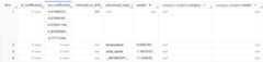
   The results should look similar to the following:

   

   Thenon_seasonal_p,non_seasonal_d,non_seasonal_q, andhas_driftoutput columns define an ARIMA model in the training pipeline. Thelog_likelihood,AIC, andvarianceoutput columns are relevant to the ARIMAmodel fitting process.

   Theauto.ARIMA algorithm uses theKPSS test to determine the best valuefornon_seasonal_d, which in this case is1. Whennon_seasonal_d is1,theauto.ARIMA algorithm trains 42 different candidate ARIMA models in parallel.In this example, all 42 candidate models are valid, so the output contains 42rows, one for each candidate ARIMA model; in cases where some of the modelsaren't valid, they are excluded from the output. These candidate models arereturned in ascending order by AIC. The model in the first row has the lowestAIC, and is considered the best model. The best model is saved as the finalmodel and is used when you call functions such asML.FORECAST on the model.

   Theseasonal_periods column contains information about the seasonal patternidentified in the time series data. It has nothing to do with the ARIMAmodeling, therefore it has the same value across all output rows. It reports aweekly pattern, which agrees with the results you saw if you chose tovisualize the input data.

   Thehas_holiday_effect,has_spikes_and_dips, andhas_step_changes columnsprovide information about the input time series data, and are not related tothe ARIMA modeling. These columns are returned because the value of thedecompose_time_series option in theCREATE MODEL statement isTRUE.These columns also have the same values across all output rows.

   Theerror_message column shows any errors that incurred during theauto.ARIMA fitting process. One possible reason for errors is when the selectednon_seasonal_p,non_seasonal_d,non_seasonal_q, andhas_drift columnsare not able to stabilize the time series. To retrieve the errormessage of all the candidate models, set theshow_all_candidate_modelsoption toTRUE when you create the model.

   For more information about the output columns, seeML.ARIMA_EVALUATE function.

Inspect the model's coefficients

Inspect the time series model's coefficients by using theML.ARIMA_COEFFICIENTS function.

Follow these steps to retrieve the model's coefficients:

1. In the Google Cloud console, go to theBigQuery page.

   Go to BigQuery

2. In the query editor, paste in the following query and clickRun:

   SELECT*FROMML.ARIMA_COEFFICIENTS(MODEL`bqml_tutorial.seattle_pm25_xreg_model`);

   The results should look similar to the following:

   

   Thear_coefficients output column shows the model coefficients of theautoregressive (AR) part of the ARIMA model. Similarly, thema_coefficientsoutput column shows the model coefficients of the moving-average (MA) part ofthe ARIMA model. Both of these columns contain array values, whose lengths areequal tonon_seasonal_p andnon_seasonal_q, respectively. You saw in theoutput of theML.ARIMA_EVALUATE function that the best model has anon_seasonal_p value of0 and anon_seasonal_q value of5. Therefore, intheML.ARIMA_COEFFICIENTS output, thear_coefficients value is an emptyarray and thema_coefficients value is a 5-element array. Theintercept_or_drift value is the constant term in the ARIMA model.

   Theprocessed_input,weight, andcategory_weights output column show theweights for each feature and the intercept in the linear regression model. Ifthe feature is a numerical feature, the weight is in theweight column. If thefeature is a categorical feature, thecategory_weights value is an array ofstruct values, where each struct value contains the name and weight of a givencategory.

   For more information about the output columns, seeML.ARIMA_COEFFICIENTS function.

Use the model to forecast data

Forecast future time series values by using theML.FORECASTfunction.

In the following GoogleSQL query, theSTRUCT(30 AS horizon, 0.8 AS confidence_level) clause indicates that thequery forecasts 30 future time points, and generates a prediction intervalwith a 80% confidence level.

Follow these steps to forecast data with the model:

1. In the Google Cloud console, go to theBigQuery page.

   Go to BigQuery

2. In the query editor, paste in the following query and clickRun:

   SELECT*FROMML.FORECAST(MODEL`bqml_tutorial.seattle_pm25_xreg_model`,STRUCT(30AShorizon,0.8ASconfidence_level),(SELECTdate,temperature,wind_speedFROM`bqml_tutorial.seattle_air_quality_daily`WHEREdate>DATE('2020-12-31')));

   The results should look similar to the following:

   

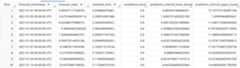
   The output rows are in chronological order by theforecast_timestamp column value. In time series forecasting, the predictioninterval, as represented by theprediction_interval_lower_bound andprediction_interval_upper_bound column values, is as important as theforecast_value column value. Theforecast_value value is the middle pointof the prediction interval. The prediction interval depends on thestandard_error andconfidence_level column values.

   For more information about the output columns, seeML.FORECAST function.

Evaluate forecasting accuracy

Evaluate the forecasting accuracy of the model by using theML.EVALUATEfunction.

In the following GoogleSQL query, the secondSELECT statementprovides the data with the future features, which are usedto forecast the future values to compare to the actual data.

Follow these steps to evaluate the model's accuracy:

1. In the Google Cloud console, go to theBigQuery page.

   Go to BigQuery

2. In the query editor, paste in the following query and clickRun:

   SELECT*FROMML.EVALUATE(MODEL`bqml_tutorial.seattle_pm25_xreg_model`,(SELECTdate,pm25,temperature,wind_speedFROM`bqml_tutorial.seattle_air_quality_daily`WHEREdate>DATE('2020-12-31')),STRUCT(TRUEASperform_aggregation,30AShorizon));

   The results should look similar the following:

   

   For more information about the output columns, seeML.EVALUATE function.

Explain the forecasting results

You can get explainability metrics in addition to forecast data by using theML.EXPLAIN_FORECAST function. TheML.EXPLAIN_FORECAST function forecastsfuture time series values and also returns all the separate components of thetime series.

Similar to theML.FORECAST function, theSTRUCT(30 AS horizon, 0.8 AS confidence_level) clause used in theML.EXPLAIN_FORECAST function indicates that the query forecasts 30 futuretime points and generates a prediction interval with 80% confidence.

Follow these steps to explain the model's results:

1. In the Google Cloud console, go to theBigQuery page.

   Go to BigQuery

2. In the query editor, paste in the following query and clickRun:

   SELECT*FROMML.EXPLAIN_FORECAST(MODEL`bqml_tutorial.seattle_pm25_xreg_model`,STRUCT(30AShorizon,0.8ASconfidence_level),(SELECTdate,temperature,wind_speedFROM`bqml_tutorial.seattle_air_quality_daily`WHEREdate>DATE('2020-12-31')));

   The results should look similar to the following:

   

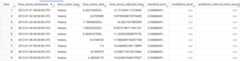
   The output rows are ordered chronologically by thetime_series_timestampcolumn value.

   For more information about the output columns, seeML.EXPLAIN_FORECAST function.