Numerical data: Normalization

Page Summary
Data normalization is crucial for enhancing machine learning model performance by scaling features to a similar range.
Linear scaling, Z-score scaling, and log scaling are common normalization techniques, each suitable for different data distributions.
Clipping helps manage outliers by limiting extreme values within a defined range, improving model robustness.
Selecting the appropriate normalization method depends on the specific dataset and feature characteristics, often requiring experimentation for optimal results.
Applying normalization consistently during both training and prediction stages ensures accurate and reliable model outcomes.
After examining your data through statistical and visualization techniques,you should transform your data in ways that will help your model train moreeffectively. The goal ofnormalization is to transformfeatures to be on a similar scale. For example, consider the following twofeatures:
- Feature
Xspans the range 154 to 24,917,482. - Feature
Yspans the range 5 to 22.
These two features span very different ranges. Normalization might manipulateX andY so that they span a similar range, perhaps 0 to 1.
Normalization provides the following benefits:
- Helps modelsconverge more quickly during training.When different features have different ranges, gradient descent can"bounce" and slow convergence. That said, more advanced optimizers likeAdagradandAdam protect against this problem bychanging the effective learning rate over time.
- Helps modelsinfer better predictions.When different features have different ranges, the resultingmodel might make somewhat less useful predictions.
- Helpsavoid the "NaN trap" when feature values are very high.NaN is an abbreviation fornot a number. When a value in a model exceeds thefloating-point precision limit, the system sets the value to
NaNinsteadof a number. When one number in the model becomes a NaN, other numbers inthe model also eventually become a NaN. - Helps the modellearn appropriate weights for each feature.Without feature scaling, the model pays too much attentionto features with wide ranges and not enough attention to features withnarrow ranges.
We recommend normalizing numeric features covering distinctlydifferent ranges (for example, age and income).We also recommend normalizing a single numeric feature that covers a wide range,such ascity population.
Consider the following two features:
- Feature
A's lowest value is -0.5 and highest is +0.5. - Feature
B's lowest value is -5.0 and highest is +5.0.
FeatureA and FeatureB have relatively narrow spans. However, FeatureB'sspan is 10 times wider than FeatureA's span. Therefore:
- At the start of training, the model assumes that Feature
Bis ten timesmore "important" than FeatureA. - Training will take longer than it should.
- The resulting model may be suboptimal.
The overall damage due to not normalizing will be relatively small; however,we still recommend normalizing Feature A and Feature B to the same scale,perhaps -1.0 to +1.0.
Now consider two features with a greater disparity of ranges:
- Feature
C's lowest value is -1 and highest is +1. - Feature
D's lowest value is +5000 and highest is +1,000,000,000.
If you don't normalize FeatureC and FeatureD, your model will likelybe suboptimal. Furthermore, training will take much longer toconverge or even fail to converge entirely!
This section covers three popular normalization methods:
- linear scaling
- Z-score scaling
- log scaling
This section additionally coversclipping. Although not a truenormalization technique, clipping does tame unruly numerical features intoranges that produce better models.
Linear scaling
Linear scaling (more commonlyshortened to justscaling) means converting floating-point values fromtheir natural range into a standard range—usually 0 to 1 or-1 to +1.
Click the icon to see the math.
Use the following formula to scale to the standard range0 to 1, inclusive:
$$ x' = (x - x_{min}) / (x_{max} - x_{min}) $$where:
- $x'$ is the scaled value.
- $x$ is the original value.
- $x_{min}$ is the lowest value in the dataset of this feature.
- $x_{max}$ is the highest value in the dataset of this feature.
For example, consider a feature namedquantity whose naturalrange spans 100 to 900. Suppose the natural value ofquantity in aparticular example is 300. Therefore, you can calculate the normalized valueof 300 as follows:
- $x$ = 300
- $x_{min}$ = 100
- $x_{max}$ = 900
x' = (300 - 100) / (900 - 100)x' = 200 / 800x' = 0.25
Linear scaling is a good choice when all of the following conditions are met:
- The lower and upper bounds of your data don't change much over time.
- The feature contains few or no outliers, and those outliers aren'textreme.
- The feature is approximately uniformly distributed across its range.That is, a histogram would show roughly even bars for most values.
Suppose humanage is a feature. Linear scaling is a good normalizationtechnique forage because:
- The approximate lower and upper bounds are 0 to 100.
agecontains a relatively small percentage of outliers. Only about 0.3% ofthe population is over 100.- Although certain ages are somewhat better represented than others, a largedataset should contain sufficient examples of all ages.
Exercise: Check your understanding
Suppose your model has a feature namednet_worth that holds the networth of different people. Would linear scaling be a good normalizationtechnique fornet_worth? Why or why not?Click the icon to see the answer.
Answer: Linear scaling would be a poor choice for normalizingnet_worth. This feature contains many outliers, and the valuesare not uniformly distributed across its primary range. Most people wouldbe squeezed within a very narrow band of the overall range.
Z-score scaling
AZ-score is the number of standard deviations a value is from the mean.For example, a value that is 2 standard deviationsgreater than the meanhas a Z-score of +2.0. A value that is 1.5 standard deviationsless thanthe mean has a Z-score of -1.5.
Representing a feature withZ-score scaling means storing that feature'sZ-score in the feature vector. For example, the following figure shows twohistograms:
- On the left, a classic normal distribution.
- On the right, the same distribution normalized by Z-score scaling.

Z-score scaling is also a good choice for data like that shown inthe following figure, which has only a vaguely normal distribution.
Click the icon to see the math.
Use the following formula to normalize a value, $x$, toits Z-score:
$$ x' = (x - μ) / σ $$where:
- $x'$ is the Z-score.
- $x$ is the raw value; that is, $x$ is the value you are normalizing.
- $μ$ is the mean.
- $σ$ is the standard deviation.
For example, suppose:
- mean = 100
- standard deviation = 20
- original value = 130
Therefore:
Z-score = (130 - 100) / 20 Z-score = 30 / 20 Z-score = +1.5
Click the icon to learn more about normal distributions.
In a classic normal distribution:
- At least 68.27% of data has a Z-score between -1.0 and +1.0.
- At least 95.45% of data has a Z-score between -2.0 and +2.0.
- At least 99.73% of data has a Z-score between -3.0 and +3.0.
- At least 99.994% of data has a Z-score between -4.0 and +4.0.
Z-score is a good choice when the data follows a normal distribution ora distribution somewhat like a normal distribution.
Note that some distributions might be normal within the bulk of theirrange, but still contain extreme outliers. For example, nearly all of thepoints in anet_worth feature might fit neatly into 3 standard deviations,but a few examples of this feature could be hundreds of standard deviationsaway from the mean. In these situations, you can combine Z-score scaling withanother form of normalization (usually clipping) to handle this situation.
Exercise: Check your understanding
Suppose your model trains on a feature namedheight that holds the adultheights of ten million women. Would Z-score scaling be a good normalizationtechnique forheight? Why or why not?Click the icon to see the answer.
Answer: Z-score scaling would be a good normalization techniqueforheight because this feature conforms to a normal distribution.Ten million examples implies a lot of outliers—probably enough outliers forthe model to learn patterns on very high or very low Z-scores.
Log scaling
Log scaling computes the logarithm of the raw value. In theory, thelogarithm could be any base; in practice, log scaling usually calculatesthe natural logarithm (ln).
Click the icon to see the math.
Use the following formula to normalize a value, $x$, toits log:
$$ x' = ln(x) $$where:
- $x'$ is the natural logarithm of $x$.
- original value = 54.598
Therefore, the log of the original value is about 4.0:
4.0 = ln(54.598)
Log scaling is helpful when the data conforms to apower law distribution.Casually speaking, a power law distribution looks as follows:
- Low values of
Xhave very high values ofY. - As the values of
Xincrease, the values ofYquickly decrease.Consequently, high values ofXhave very low values ofY.
Movie ratings are a good example of a power law distribution. In the followingfigure, notice:
- A few movies have lots of user ratings. (Low values of
Xhave highvalues ofY.) - Most movies have very few user ratings. (High values of
Xhave lowvalues ofY.)
Log scaling changes the distribution, which helps train a model that willmake better predictions.

As a second example, book sales conform to a power law distribution because:
- Most published books sell a tiny number of copies, maybe one or two hundred.
- Some books sell a moderate number of copies, in the thousands.
- Only a fewbestsellers will sell more than a million copies.
Suppose you are training a linear model to find the relationshipof, say, book covers to book sales. A linear model training on raw values wouldhave to find something about book covers on books that sell a million copiesthat is 10,000 more powerful than book covers that sell only 100 copies.However, log scaling all the sales figures makes the task far more feasible.For example, the log of 100 is:
~4.6 = ln(100)
while the log of 1,000,000 is:
~13.8 = ln(1,000,000)
So, the log of 1,000,000 is only about three times larger than the log of 100.You probablycould imagine a bestseller book cover being about three timesmore powerful (in some way) than a tiny-selling book cover.
Clipping
Clipping is a technique tominimize the influence of extreme outliers. In brief, clipping usually caps(reduces) the value of outliers to a specific maximum value. Clipping is astrange idea, and yet, it can be very effective.
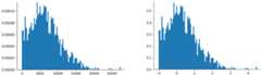
For example, imagine a dataset containing a feature namedroomsPerPerson,which represents the number of rooms (total rooms dividedby number of occupants) for various houses. The following plot shows that over99% of the feature values conform to a normal distribution (roughly, a mean of1.8 and a standard deviation of 0.7). However, the feature containsa few outliers, some of them extreme:

How can you minimize the influence of those extreme outliers? Well, thehistogram is not an even distribution, a normal distribution, or a power lawdistribution. What if you simplycap orclip the maximum value ofroomsPerPerson at an arbitrary value, say 4.0?

Clipping the feature value at 4.0 doesn't mean that your model ignores allvalues greater than 4.0. Rather, it means that all values that were greaterthan 4.0 now become 4.0. This explains the peculiar hill at 4.0. Despitethat hill, the scaled feature set is now more useful than the original data.
Wait a second! Can you really reduce every outlier value to some arbitrary upperthreshold? When training a model, yes.
You can also clip values after applying other forms of normalization.For example, suppose you use Z-score scaling, but a few outliers haveabsolute values far greater than 3. In this case, you could:
- Clip Z-scores greater than 3 to become exactly 3.
- Clip Z-scores less than -3 to become exactly -3.
Clipping prevents your model from overindexing on unimportant data. However,some outliers are actually important, so clip values carefully.
Summary of normalization techniques
The best normalization technique is one that works well in practice, so try new ideas if you think they'll work well on your feature distribution.| Normalization technique | Formula | When to use |
|---|---|---|
| Linear scaling | $$ x' = \frac{x - x_{min}}{x_{max} - x_{min}} $$ | When the feature is mostly uniformly distributed across range.Flat-shaped |
| Z-score scaling | $$ x' = \frac{x - μ}{σ}$$ | When the feature is normally distributed (peak close to mean).Bell-shaped |
| Log scaling | $$ x' = log(x)$$ | When the feature distribution is heavy skewed on at least either side of tail.Heavy Tail-shaped |
| Clipping | If $x > max$, set $x' = max$ If $x< min$, set $x' = min$ | When the feature contains extreme outliers. |
Exercise: Test your knowledge

Suppose you are developing a model that predicts a data center's productivity based on the temperature measured inside the data center. Almost all of thetemperature values in your dataset fall between 15 and 30 (Celsius), with the following exceptions:
- Once or twice per year, on extremely hot days, a few values between 31 and 45 are recorded in
temperature. - Every 1,000th point in
temperatureis set to 1,000 rather than the actual temperature.
Which would be a reasonable normalization technique fortemperature?
The values of 1,000 are mistakes, and should be deleted rather than clipped.
The values between 31 and 45 are legitimate data points. Clipping would probably be a good idea for these values, assuming the dataset doesn't contain enough examples in this temperature range to train the model to make good predictions. However, during inference, note that the clipped model would therefore make the same prediction for a temperature of 45 as for a temperature of 35.
Except as otherwise noted, the content of this page is licensed under theCreative Commons Attribution 4.0 License, and code samples are licensed under theApache 2.0 License. For details, see theGoogle Developers Site Policies. Java is a registered trademark of Oracle and/or its affiliates.
Last updated 2025-12-03 UTC.