
GIFT tutorial for advanced users
Pierre Denelle& Patrick Weigelt
2024-12-02
Source:vignettes/GIFT_advanced_users.RmdGIFT_advanced_users.Rmd![]()

This vignette documents some functions and specificities that werenot presented in themainvignette of the package. It is mainly intended for advanced users ofthe GIFT database.
1. Versions and metadata for checklists
All functions in the package have aversion argument.This argument allows you to retrieve different instances of the GIFTdatabase and thus make all previous studies using the GIFT databasereproducible. For example, the version used in Weigelt et al. (2020) is"1.0". To get more information about the contents of thedifferent versions, you can gohere and click on theVersion Log tab.
To access all the available versions of the database, you can run thefollowing function:
versions<-GIFT_versions()kable(versions,"html")%>%kable_styling(full_width=FALSE)| ID | version | description | taxonomy | phylogeny | overlap |
|---|---|---|---|---|---|
| 1 | 1.0 | 2018-08-08: Data included in and workflows used to assemble GIFT 1.0 aredescribed in detail in: Weigelt, P., König, C. & Kreft, H. (2020)GIFT – A Global Inventory of Floras and Traits for macroecology andbiogeography. Journal of Biogeography, 47, 16-43. doi: 10.1111/jbi.13623 | The Plant List 1.1 and resources used by TNRS at the time | NA | gaptani (version: okt2005, ID_column: UNITID); glonaf (version:2017-06-12; ID_column: OBJIDsic); gmba (version: 1.0, ID_column:rownames) |
| 2 | 2.0 | 2019-09-01: New checklist and trait data included for Europe, theMediterranean, temperate Asia, Panama, Japan, Java, New Zealand, EasterIsland and the Torres Strait Islands. Updated workflows to documentbiases in the distribution of trait data; Updated taxonomic traitderivation; Final trait values and agreement scores for trait valuesfrom several resources are now calculated separately including andexcluding restricted resources. | The Plant List 1.1 and resources used by TNRS at the time | NA | gaptani (version: okt2005, ID_column: UNITID); glonaf (version:2017-06-12; ID_column: OBJIDsic); gmba (version: 1.0, ID_column:rownames) |
| 3 | 2.1 | 2021-05-21: New checklists and traits included for the Americas, Crimea,Madagascar, Arabian peninsula, Laos, Bhutan, India, China, Sunda-Sahulshelf, Tonga, Canary Islands, West Africa and for ferns and palmsglobally. Large categorical trait data included from Try. | The Plant List 1.1 and resources used by TNRS at the time | NA | gaptani (version: okt2005, ID_column: UNITID); glonaf (version:2017-06-12; ID_column: OBJIDsic); gmba (version: 1.0, ID_column:rownames) |
| 4 | 2.2 | 2022-05-30: New checklists (with a focus on endemic species) and traitsfor various oceanic archipelagos (Cook Islands, Madeira, Arctic Islands,Cayman Islands, Comores, Juan Fernandez, Palau, Galapagos, FrisianIslands, Antilles, Japan, Mayotte, Fiji, Taiwan, etc.) and variousmainland regions (Equatorial Guinea and the entire former USSR insub-regions). | The Plant List 1.1 and resources used by TNRS at the time | NA | gaptani (version: okt2005, ID_column: UNITID); glonaf (version:2017-06-12; ID_column: OBJIDsic); gmba (version: 1.0, ID_column:rownames) |
| 5 | 3.0 | 2023-06-30: New data and updated workflows as described in: Denelle, P.,Weigelt, P. & Kreft, H. (2023) GIFT - an R package to access theGlobal Inventory of Floras and Traits. BioRxiv, doi:10.1101/2023.06.27.546704. Updated workflows include: (1) New taxonomicname standardization based on WCVP; (2) More statistics on species leveltrait aggregation; (3) Updated extraction of raster layer values perGIFT region and new raster resources; (4) Updated phylogeny. | World Checklist of Vascular Plants (WCVP, v9) and resources used by TNRSat the time | Phylogeny built using U.PhyloMaker R-package (Jin & Qian, 2022)based on the GBOTB megatree from Smith & Brown (2018) and Zanne etal. (2014), standardized according to WCVP. | gaptani (version: okt2005, ID_column: UNITID); glonaf (version:2021-07-02; ID_column: OBJIDsic); gmba (version: 1.2, ID_column:rownames) |
| 6 | 3.1 | 2023-11-11: New checklist data for Mongolia and Farasan Archipelago andcorrection of seed traits for Hawaii (ref 16; units). | World Checklist of Vascular Plants (WCVP, v9) and resources used by TNRSat the time | Phylogeny built using U.PhyloMaker R-package (Jin & Qian, 2022)based on the GBOTB megatree from Smith & Brown (2018) and Zanne etal. (2014), standardized according to WCVP. | gaptani (version: okt2005, ID_column: UNITID); glonaf (version:2021-07-02; ID_column: OBJIDsic); gmba (version: 2.0, ID_column:GMBA_V2_ID) |
| 7 | 3.2 | 2024-06-13: New oceanic archipelago trait data and global parasitisminformation | World Checklist of Vascular Plants (WCVP, v9) and resources used by TNRSat the time | Phylogeny built using U.PhyloMaker R-package (Jin & Qian, 2022)based on the GBOTB megatree from Smith & Brown (2018) and Zanne etal. (2014), standardized according to WCVP. | gaptani (version: okt2005, ID_column: UNITID); glonaf (version:2021-07-02; ID_column: OBJIDsic); gmba (version: 2.0, ID_column:GMBA_V2_ID) |
Theversion column of this table is the one to use ifyou want to retrieve past versions of the GIFT database. By default, theargument used isGIFT_version = "latest" which leads to thecurrent latest stable version of the database (“2.0” in October2022).
TheGIFT_lists() function can be run to retrievemetadata about the GIFT checklists. In the next chunk, we call it withdifferent values for theGIFT_version argument.
list_latest<-GIFT_lists(GIFT_version="latest")# default valuelist_1<-GIFT_lists(GIFT_version="1.0")The number of available checklists was 3122 in the version 1.0 andequals 4475 in the version 2.0.
2. References
When using the GIFT database in a research article, it is a goodpractice to cite the references used, and list them in an Appendix. Thefollowing function retrieves the reference for each checklist, as wellas some metadata. References are documented in theref_longcolumn.
ref<-GIFT_references()ref<-ref[which(ref$ref_ID%in%c(22,10333,10649)),c("ref_ID","ref_long","geo_entity_ref")]# 3 first rows of that tablekable(ref,"html")%>%kable_styling(full_width=FALSE)| ref_ID | ref_long | geo_entity_ref | |
|---|---|---|---|
| 22 | 22 | Kirchner, Picot, Merceron & Gigot (2010) Flore vasculaire de LaRéunion. Conservatoire Botanique National de Mascarin, Réunion; France. | La Réunion |
| 667 | 10333 | Zizka (1991) Flowering plants of Easter Island. Palmarum hortusfrancofurtensis 3, 3-108. | Easter Island |
| 880 | 10649 | Pavlov (1954-1966) Flora Kazakhstana. Nauka Kazakhskoy SSR, Alma-Ata,Kazakhstan. | Kazakhstan |
The next chunk describes the steps to retrieve the publicationsources when you start from specific regions, let’s say the Canaryislands.
# List of all regionsregions<-GIFT_regions()# Examplecan<-1036# entity ID for Canary islands# What referencesgift_lists<-GIFT_lists()can_ref<-gift_lists[which(gift_lists$entity_ID%in%c(can)),"ref_ID"]# What sourceskable(ref[which(ref$ref_ID%in%can_ref),],"html")%>%kable_styling(full_width=TRUE)| ref_ID | ref_long | geo_entity_ref |
|---|---|---|
3. Checklist data
The main wrapper function for retrieving checklists and their speciescomposition isGIFT_checklists() but you can also retrieveindividual checklists usingGIFT_checklists_raw(). Youwould need to know the identification numberlist_ID of thechecklists you want to retrieve.
To quickly see all thelist_ID available in the database, you can runGIFT_lists() as shown inSection1.
When callingGIFT_checklists_raw(), you can set theargumentnamesmatched toTRUE in order to getadditional columns informing about the taxonomic harmonization that wasperformed when the list was uploaded to the GIFT database.
listID_1<-GIFT_checklists_raw(list_ID=c(11926))listID_1_tax<-GIFT_checklists_raw(list_ID=c(11926), namesmatched=TRUE)ncol(listID_1)# 16 columnsncol(listID_1_tax)# 33 columnslength(unique(listID_1$work_ID));length(unique(listID_1_tax$orig_ID))In the list we called up, you can see that we “lost” some speciesafter the taxonomic harmonization since we went from 1331 in the sourceto 1106 after the taxonomic harmonization. This means that severalspecies were considered as synonyms or unknown plant species in thetaxonomic backbone used for harmonization.
Note: the mainservice used for taxonomic harmonization of species nameswasThe Plant List up to version 2.0 and World checklist of VascularPlantsafterwards.
4. Spatial subset
In themainvignette, we illustrated how to retrieve checklists that fall into aprovided shapefile, using the western Mediterranean basin provided withthe GIFT R package.
data("western_mediterranean")Here we provide more details on the different values theoverlap argument can take, using theGIFT_spatial() function. The following figure illustrateshow this argument works:

Figure 1. GIFT spatial
We now illustrate this by retrieving checklists falling in thewestern Mediterranean basin using the four options available.
med_centroid_inside<-GIFT_spatial(shp=western_mediterranean, overlap="centroid_inside")med_extent_intersect<-GIFT_spatial(shp=western_mediterranean, overlap="extent_intersect")med_shape_intersect<-GIFT_spatial(shp=western_mediterranean, overlap="shape_intersect")med_shape_inside<-GIFT_spatial(shp=western_mediterranean, overlap="shape_inside")length(unique(med_extent_intersect$entity_ID))length(unique(med_shape_intersect$entity_ID))length(unique(med_centroid_inside$entity_ID))length(unique(med_shape_inside$entity_ID))We see here that we progressively lose lists as we apply moreselective criterion on the spatial overlap. The most restrictive optionbeingoverlap = "shape_inside" with 72 regions, thenoverlap = "centroid_inside" with 84 regions,overlap = "shape_intersect" with 104 regions and finallythe less restrictive one beingoverlap = "extent_intersect"with 108 regions.
Using the functionsGIFT_shapes()and calling it for the entity_IDs retrieved in each instance, we candownload the shape files for each region.
geodata_extent_intersect<-GIFT_shapes(med_extent_intersect$entity_ID)geodata_shape_inside<-geodata_extent_intersect[which(geodata_extent_intersect$entity_ID%in%med_shape_inside$entity_ID),]geodata_centroid_inside<-geodata_extent_intersect[which(geodata_extent_intersect$entity_ID%in%med_centroid_inside$entity_ID),]geodata_shape_intersect<-geodata_extent_intersect[which(geodata_extent_intersect$entity_ID%in%med_shape_intersect$entity_ID),]And then make a map.
par_overlap<-par(mfrow=c(2,2), mai=c(0,0,0.5,0))plot(sf::st_geometry(geodata_shape_inside), col=geodata_shape_inside$entity_ID, main=paste("shape inside\n",length(unique(med_shape_inside$entity_ID)),"polygons"))plot(sf::st_geometry(western_mediterranean), lwd=2, add=TRUE)plot(sf::st_geometry(geodata_centroid_inside), col=geodata_centroid_inside$entity_ID, main=paste("centroid inside\n",length(unique(med_centroid_inside$entity_ID)),"polygons"))points(geodata_centroid_inside$point_x,geodata_centroid_inside$point_y)plot(sf::st_geometry(western_mediterranean), lwd=2, add=TRUE)plot(sf::st_geometry(geodata_shape_intersect), col=geodata_shape_intersect$entity_ID, main=paste("shape intersect\n",length(unique(med_shape_intersect$entity_ID)),"polygons"))plot(sf::st_geometry(western_mediterranean), lwd=2, add=TRUE)plot(sf::st_geometry(geodata_extent_intersect), col=geodata_extent_intersect$entity_ID, main=paste("extent intersect\n",length(unique(med_extent_intersect$entity_ID)),"polygons"))plot(sf::st_geometry(western_mediterranean), lwd=2, add=TRUE)par(par_overlap)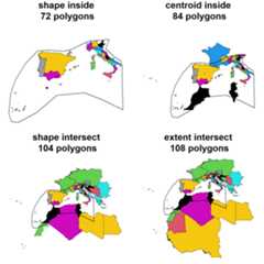
5. Remove overlapping regions
GIFT comprises many polygons and for some regions, there are severalpolygons overlapping. How to remove overlapping polygons and theassociated parameters are two things detailed in themainvignette. We here provide further details:
length(med_shape_inside$entity_ID)## [1] 72length(GIFT_no_overlap(med_shape_inside$entity_ID, area_threshold_island=0, area_threshold_mainland=100, overlap_threshold=0.1))## [1] 53# The following polygons are overlapping:GIFT_no_overlap(med_shape_inside$entity_ID, area_threshold_island=0, area_threshold_mainland=100, overlap_threshold=0.1)## [1] 145 146 147 148 149 150 151 414 415 416 417 547## [13] 548 549 550 551 552 586 591 592 736 738 739 10001## [25] 10072 10104 10184 10303 10422 10430 10978 11029 11030 11031 11033 11035## [37] 11038 11039 11042 11044 11045 11046 11434 11474 11477 11503 12231 12232## [49] 12233 12632 12633 12634 12635# Example of two overlapping polygons: Spain mainland and Andalusiaoverlap_shape<-GIFT_shapes(entity_ID=c(10071,12078))par_overlap_shp<-par(mfrow=c(1,1))plot(sf::st_geometry(overlap_shape), col=c(rgb(red=1, green=0, blue=0, alpha=0.5),rgb(red=0, green=0, blue=1, alpha=0.3)), lwd=c(2,1), main="Overlapping polygons")
par(par_overlap_shp)GIFT_no_overlap(c(10071,12078), area_threshold_island=0, area_threshold_mainland=100, overlap_threshold=0.1)## [1] 12078GIFT_no_overlap(c(10071,12078), area_threshold_island=0, area_threshold_mainland=100000, overlap_threshold=0.1)## [1] 100715.2. By ref_ID
InGIFT_checklists(), there is also the possibility toremove overlapping polygons only if they belong to the same reference(i.e. sameref_ID).
We show how this works with the following example:
ex<-GIFT_checklists(taxon_name="Tracheophyta", by_ref_ID=FALSE, list_set_only=TRUE, GIFT_version="3.0")ex2<-GIFT_checklists(taxon_name="Tracheophyta", remove_overlap=TRUE, by_ref_ID=TRUE, list_set_only=TRUE, GIFT_version="3.0")ex3<-GIFT_checklists(taxon_name="Tracheophyta", remove_overlap=TRUE, by_ref_ID=FALSE, list_set_only=TRUE, GIFT_version="3.0")length(unique(ex$lists$ref_ID))# 369 checklistslength(unique(ex2$lists$ref_ID))# 364 checklistslength(unique(ex3$lists$ref_ID))# 336 checklistsAsking for checklists of vascular plants, we get 369 checklistswithout any overlapping criterion, 336 if we remove overlapping polygonsand 364 if we remove overlapping polygons at the reference level.
So what is the difference between the second and third case?
Let’s look at the checklists that are present in the second example butnot in the third.
28 references are in the second example (overlapping regions removedat the reference level) and not in the third (all overlapping regionsremoved). If we look at one of the listed referencesref_ID = 10143, we see that it is a checklist for thePilbara region in Australia. Itsentity_ID is 10043.Looking at the GIFT web site, we see that other regions can overlap withit.
# Pilbara region Australy and overlapping shapespilbara<-GIFT_shapes(entity_ID=c(10043,12172,11398,11391,10918))ggplot(pilbara)+geom_sf(aes(fill=as.factor(entity_ID)), alpha=0.5)+scale_fill_brewer("entity_ID", palette="Set1")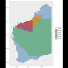
Since these polygons do not belong to the sameref_ID,they are kept ifby_ref_ID = TRUE but are removed ifby_ref_ID = FALSE.
6. Species
All the plant species present in the GIFT database can be retrievedusingGIFT_species().
species<-GIFT_species()To add additional information, like their order or family, we cancallGIFT_taxgroup().
# Add Familyspecies$Family<-GIFT_taxgroup(as.numeric(species$work_ID), taxon_lvl="family", return_ID=FALSE, species=species)Order or higher levels can also be retrieved.
GIFT_taxgroup(as.numeric(species$work_ID[1:5]), taxon_lvl="order", return_ID=FALSE)GIFT_taxgroup(as.numeric(species$work_ID[1:5]), taxon_lvl="higher_lvl", return_ID=FALSE, species=species)As mentioned above, plant species names may vary from the originalsources they come from to the finalwork_species name theyget, due to the taxonomic harmonization procedure. Looking up a speciesand the different steps of taxonomic harmonization is possible with theGIFT_species_lookup() function.
Fagus<-GIFT_species_lookup(genus="Fagus", epithet="sylvatica", namesmatched=TRUE)In this table, we can see that the first entryFagussilvatica was later changed to the accepted nameFagussylvatica.
6.2. Retrieve work_IDs for external species list
sp_list<-c("Anemone nemorosa","Fagus sylvatica")gift_sp<-GIFT_species()sapply(sp_list,function(x)grep(x,gift_sp$work_species))gift_sp[sapply(sp_list,function(x)grep(x,gift_sp$work_species)),]# With fuzzy matching# library("fuzzyjoin")# library("dplyr")sp_list<-data.frame(work_species=c("Anemona nemorosa","Fagus sylvaticaaa"))fuzz<-stringdist_join(sp_list,gift_sp, by="work_species", mode="left", ignore_case=FALSE, method="jw", max_dist=99, distance_col="dist")fuzz%>%group_by(work_species.x)%>%slice_min(order_by=dist, n=1)7. Taxonomy
The taxonomy used in GIFT database can be downloaded usingGIFT_taxonomy().
taxo<-GIFT_taxonomy()8. Overlap_GloNAF tables (and others)
Since other global databases of plant diversity exist and may bebased on different polygons, we provide a functionGIFT_overlap() than can look at the spatial overlap betweenGIFT polygons and polygons coming from other databases.
So far,only two resources are available:glonaf andgmba.glonaf stands forGlobalNaturalized Alien Flora andgmba forGlobal Mountain BiodiversityAssessment.
GIFT_overlap() returns the spatial overlap in percentfor each pairwise combination of polygons between GIFT and the otherresource.
Let’s illustrate this with the GMBA shapefile.
gmba_overlap<-GIFT_overlap(resource="gmba")kable(gmba_overlap[1:5,],"html")%>%kable_styling(full_width=FALSE)| entity_ID | gmba_ID | overlap12 | overlap21 |
|---|---|---|---|
| 12094 | 12159 | 0.1783509 | 0.7623728 |
| 12094 | 11134 | 0.0060051 | 0.9985861 |
| 12094 | 12218 | 0.1398757 | 0.7948085 |
| 12094 | 16791 | 0.0301742 | 0.9385561 |
| 12094 | 16809 | 0.0036777 | 0.9566831 |
We see that two overlap columns are returned:overlap12andoverlap21.
The first column returns the overlap between the GIFT region and theother resource. The second column returns the overlap between the otherresource and the GIFT region.
For example, if we look at the polygon 11861 of GIFT:
gmba_overlap[which(gmba_overlap$entity_ID==11861&gmba_overlap$gmba_ID==731),]## [1] entity_ID gmba_ID overlap12 overlap21## <0 rows> (or 0-length row.names)The corresponding region is the Aisen province in Chile and itoverlaps at 95% with the GMBA polygon number 731.
At the same time the GMBA polygon 731 only overlaps at 13% with theAisen province of Chile.
This is because the corresponding mountain region is larger than theGIFT region and encompasses it as we can see on this plot (the darkpolygon is the GIFT region):

9. Plotting phylogeny for a specific region
We here want to plot the phylogenetic tree of native plant speciesoccurring in Tenerife island.
# List tablegift_list<-GIFT_lists()# Tenerife data for the following list_IDs: 150, 14110, 14228# Retrieve the liststenerife<-GIFT_checklists_raw(list_ID=c(150,14110,14228))# Extract unique native species onlytenerife_sp<-tenerife[which(tenerife$native==1),]%>%dplyr::select(work_species)%>%distinct(.keep_all=TRUE)# Harmonizing species names between the species table and the phylogenytenerife_sp$work_species<-gsub(" ","_",tenerife_sp$work_species, fixed=TRUE)# Phylogenyphy<-GIFT_phylogeny()# Dropping tipstenerife_phy<-ape::keep.tip(phy, tip=phy$tip.label[(phy$tip.label%in%tenerife_sp$work_species)])plot(tenerife_phy, type="fan", cex=0.2)
References
Denelle, P., Weigelt, P., & Kreft, H. (2023). GIFT—An R packageto access the Global Inventory of Floras and Traits.Methods inEcology and Evolution, 00, 1–11.https://doi.org/10.1111/2041-210X.14213.
Weigelt, P., König, C. & Kreft, H. (2020) GIFT – A GlobalInventory of Floras and Traits for macroecology and biogeography.Journal of Biogeography,https://doi.org/10.1111/jbi.13623.