Movatterモバイル変換

Consider a supervised learning problem where we have access to labeled training examples(x^{(i)}, y^{(i)}). Neural networks give a way of defining a complex, non-linear form of hypothesesh_{W,b}(x), with parametersW,b that we can fit to our data.

To describe neural networks, we will begin by describing the simplest possible neural network, one which comprises a single “neuron.” We will use the following diagram to denote a single neuron:

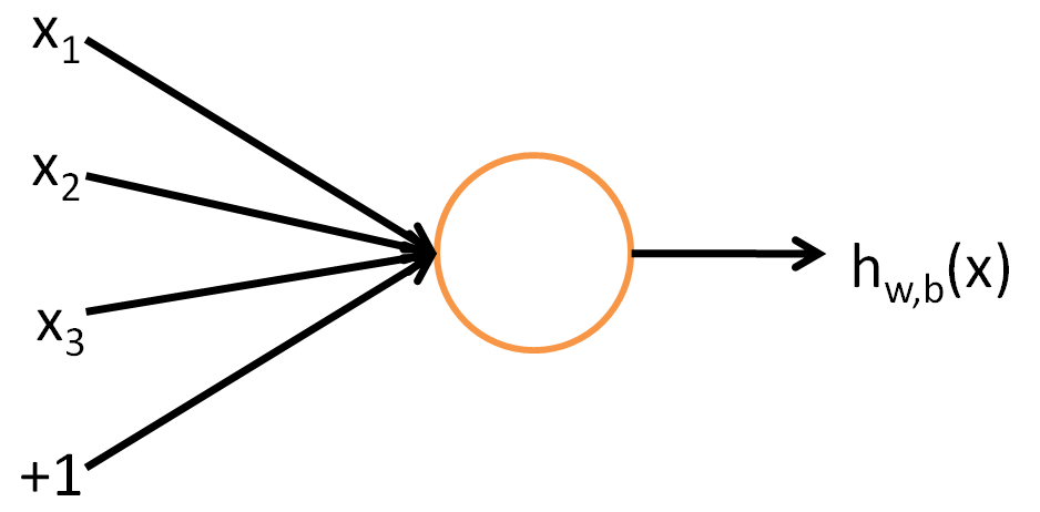
This “neuron” is a computational unit that takes as inputx_1, x_2, x_3 (and a +1 intercept term), and outputs\textstyle h_{W,b}(x) = f(W^Tx) = f(\sum_{i=1}^3 W_{i}x_i +b), wheref : \Re \mapsto \Re is called theactivation function. In these notes, we will choosef(\cdot) to be the sigmoid function:

Thus, our single neuron corresponds exactly to the input-output mapping defined by logistic regression.

Although these notes will use the sigmoid function, it is worth noting that another common choice forf is the hyperbolic tangent, or tanh, function:

Recent research has found a different activation function, the rectified linear function, often works better in practice for deep neural networks. This activation function is different from sigmoid and\tanh because it is not bounded or continuously differentiable. The rectified linear activation function is given by,

Here are plots of the sigmoid,\tanh and rectified linear functions:

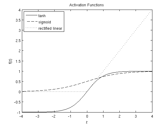
The\tanh(z) function is a rescaled version of the sigmoid, and its output range is[-1,1] instead of[0,1]. The rectified linear function is piece-wise linear and saturates at exactly 0 whenever the inputz is less than 0.

Note that unlike some other venues (including the OpenClassroom videos, and parts of CS229), we are not using the convention here ofx_0=1. Instead, the intercept term is handled separately by the parameterb.

Finally, one identity that’ll be useful later: Iff(z) = 1/(1+\exp(-z)) is the sigmoid function, then its derivative is given byf'(z) = f(z) (1-f(z)). (Iff is the tanh function, then its derivative is given byf'(z) = 1- (f(z))^2.) You can derive this yourself using the definition of the sigmoid (or tanh) function. The rectified linear function has gradient 0 whenz \leq 0 and 1 otherwise. The gradient is undefined atz=0, though this doesn’t cause problems in practice because we average the gradient over many training examples during optimization.

Neural Network model

A neural network is put together by hooking together many of our simple “neurons,” so that the output of a neuron can be the input of another. For example, here is a small neural network:

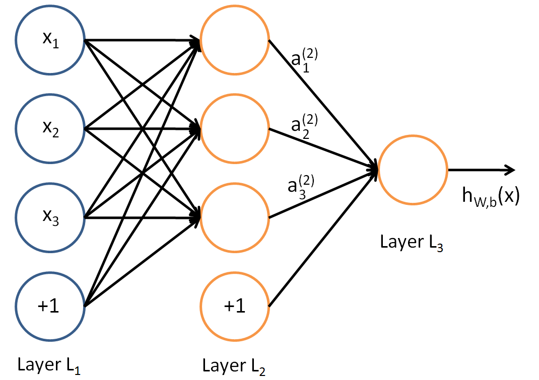
In this figure, we have used circles to also denote the inputs to the network. The circles labeled “+1” are calledbias units, and correspond to the intercept term. The leftmost layer of the network is called theinput layer, and the rightmost layer theoutput layer (which, in this example, has only one node). The middle layer of nodes is called thehidden layer, because its values are not observed in the training set. We also say that our example neural network has 3input units (not counting the bias unit), 3hidden units, and 1output unit.

We will letn_l denote the number of layers in our network; thusn_l=3 in our example. We label layerl asL_l, so layerL_1 is the input layer, and layerL_{n_l} the output layer. Our neural network has parameters(W,b) = (W^{(1)}, b^{(1)}, W^{(2)}, b^{(2)}), where we writeW^{(l)}_{ij} to denote the parameter (or weight) associated with the connection between unitj in layerl, and uniti in layerl+1. (Note the order of the indices.) Also,b^{(l)}_i is the bias associated with uniti in layerl+1. Thus, in our example, we haveW^{(1)} \in \Re^{3\times 3}, andW^{(2)} \in \Re^{1\times 3}. Note that bias units don’t have inputs or connections going into them, since they always output the value +1. We also lets_l denote the number of nodes in layerl (not counting the bias unit).

We will writea^{(l)}_i to denote theactivation (meaning output value) of uniti in layerl. Forl=1, we also usea^{(1)}_i = x_i to denote thei-th input. Given a fixed setting of the parametersW,b, our neural network defines a hypothesish_{W,b}(x) that outputs a real number. Specifically, the computation that this neural network represents is given by:

In the sequel, we also letz^{(l)}_i denote the total weighted sum of inputs to uniti in layerl, including the bias term (e.g.,\textstyle z_i^{(2)} = \sum_{j=1}^n W^{(1)}_{ij} x_j + b^{(1)}_i), so thata^{(l)}_i = f(z^{(l)}_i).

Note that this easily lends itself to a more compact notation. Specifically, if we extend the activation functionf(\cdot) to apply to vectors in an element-wise fashion (i.e.,f([z_1, z_2, z_3]) = [f(z_1), f(z_2), f(z_3)]), then we can write the equations above more compactly as:

We call this stepforward propagation. More generally, recalling that we also usea^{(1)} = x to also denote the values from the input layer, then given layerl’s activationsa^{(l)}, we can compute layerl+1’s activationsa^{(l+1)} as:

By organizing our parameters in matrices and using matrix-vector operations, we can take advantage of fast linear algebra routines to quickly perform calculations in our network.

We have so far focused on one example neural network, but one can also build neural networks with otherarchitectures (meaning patterns of connectivity between neurons), including ones with multiple hidden layers. The most common choice is a\textstyle n_l-layered network where layer\textstyle 1 is the input layer, layer\textstyle n_l is the output layer, and each layer\textstyle l is densely connected to layer\textstyle l+1. In this setting, to compute the output of the network, we can successively compute all the activations in layer\textstyle L_2, then layer\textstyle L_3, and so on, up to layer\textstyle L_{n_l}, using the equations above that describe the forward propagation step. This is one example of afeedforward neural network, since the connectivity graph does not have any directed loops or cycles.

Neural networks can also have multiple output units. For example, here is a network with two hidden layers layersL_2 andL_3 and two output units in layerL_4:

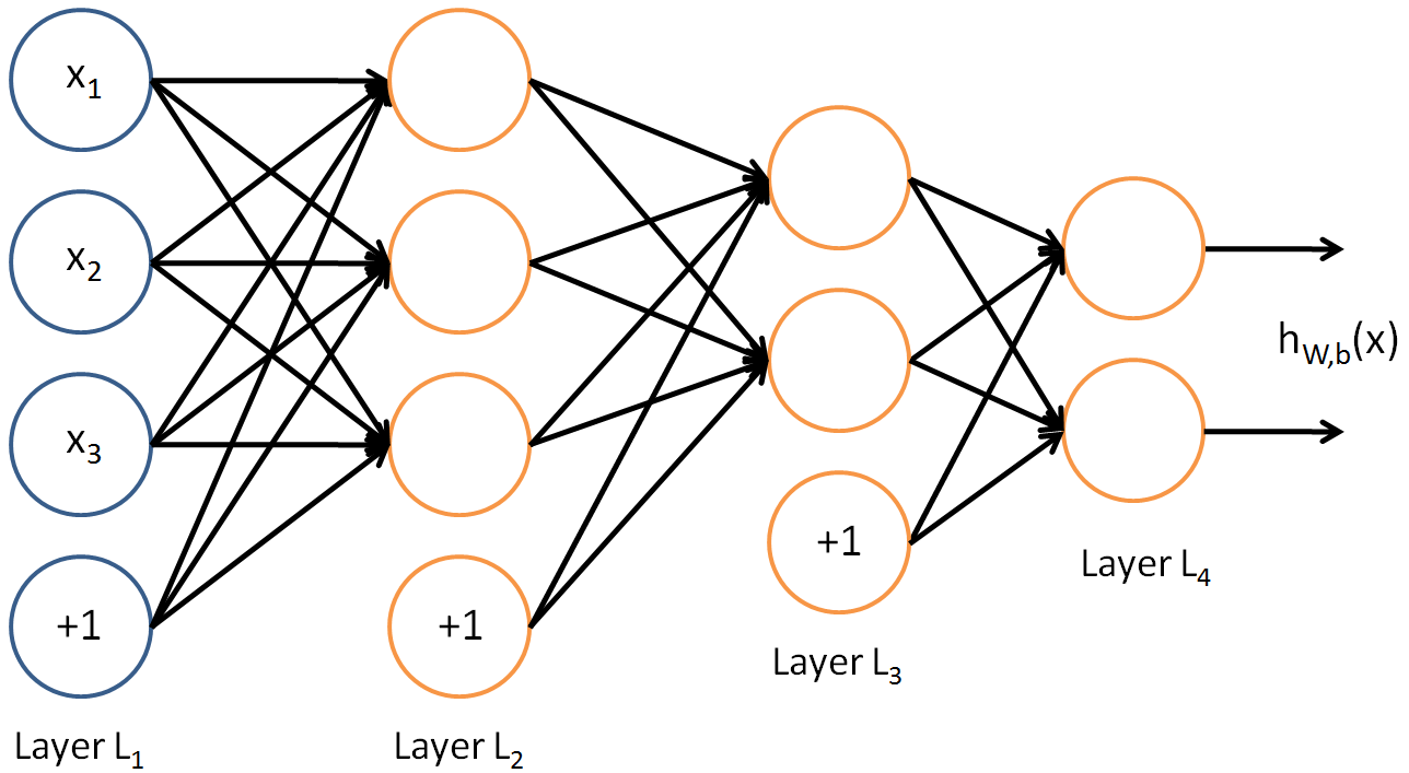
To train this network, we would need training examples(x^{(i)}, y^{(i)}) wherey^{(i)} \in \Re^2. This sort of network is useful if there’re multiple outputs that you’re interested in predicting. (For example, in a medical diagnosis application, the vectorx might give the input features of a patient, and the different outputsy_i’s might indicate presence or absence of different diseases.)

Backpropagation Algorithm

Suppose we have a fixed training set\{ (x^{(1)}, y^{(1)}), \ldots, (x^{(m)}, y^{(m)}) \} ofm training examples. We can train our neural network using batch gradient descent. In detail, for a single training example(x,y), we define the cost function with respect to that single example to be:

This is a (one-half) squared-error cost function. Given a training set ofm examples, we then define the overall cost function to be:

The first term in the definition ofJ(W,b) is an average sum-of-squares error term. The second term is a regularization term (also called aweight decay term) that tends to decrease the magnitude of the weights, and helps prevent overfitting.

(Note: Usually weight decay is not applied to the bias termsb^{(l)}_i, as reflected in our definition forJ(W, b). Applying weight decay to the bias units usually makes only a small difference to the final network, however. If you’ve taken CS229 (Machine Learning) at Stanford or watched the course’s videos on YouTube, you may also recognize this weight decay as essentially a variant of the Bayesian regularization method you saw there, where we placed a Gaussian prior on the parameters and did MAP (instead of maximum likelihood) estimation.)

Theweight decay parameter\lambda controls the relative importance of the two terms. Note also the slightly overloaded notation:J(W,b;x,y) is the squared error cost with respect to a single example;J(W,b) is the overall cost function, which includes the weight decay term.

This cost function above is often used both for classification and for regression problems. For classification, we lety = 0 or1 represent the two class labels (recall that the sigmoid activation function outputs values in[0,1]; if we were using a tanh activation function, we would instead use -1 and +1 to denote the labels). For regression problems, we first scale our outputs to ensure that they lie in the[0,1] range (or if we were using a tanh activation function, then the[-1,1] range).

Our goal is to minimizeJ(W,b) as a function ofW andb. To train our neural network, we will initialize each parameterW^{(l)}_{ij} and eachb^{(l)}_i to a small random value near zero (say according to a{Normal}(0,\epsilon^2) distribution for some small\epsilon, say0.01), and then apply an optimization algorithm such as batch gradient descent. SinceJ(W, b) is a non-convex function, gradient descent is susceptible to local optima; however, in practice gradient descent usually works fairly well. Finally, note that it is important to initialize the parameters randomly, rather than to all 0’s. If all the parameters start off at identical values, then all the hidden layer units will end up learning the same function of the input (more formally,W^{(1)}_{ij} will be the same for all values ofi, so thata^{(2)}_1 = a^{(2)}_2 = a^{(2)}_3 = \ldots for any inputx). The random initialization serves the purpose ofsymmetry breaking.

One iteration of gradient descent updates the parametersW,b as follows:

where\alpha is the learning rate. The key step is computing the partial derivatives above. We will now describe thebackpropagation algorithm, which gives an efficient way to compute these partial derivatives.

We will first describe how backpropagation can be used to compute\textstyle \frac{\partial}{\partial W_{ij}^{(l)}} J(W,b; x, y) and\textstyle \frac{\partial}{\partial b_{i}^{(l)}} J(W,b; x, y), the partial derivatives of the cost functionJ(W,b;x,y) defined with respect to a single example(x,y). Once we can compute these, we see that the derivative of the overall cost functionJ(W,b) can be computed as:

The two lines above differ slightly because weight decay is applied toW but notb.

The intuition behind the backpropagation algorithm is as follows. Given a training example(x,y), we will first run a “forward pass” to compute all the activations throughout the network, including the output value of the hypothesish_{W,b}(x). Then, for each nodei in layerl, we would like to compute an “error term”\delta^{(l)}_i that measures how much that node was “responsible” for any errors in our output. For an output node, we can directly measure the difference between the network’s activation and the true target value, and use that to define\delta^{(n_l)}_i (where layern_l is the output layer). How about hidden units? For those, we will compute\delta^{(l)}_i based on a weighted average of the error terms of the nodes that usesa^{(l)}_i as an input. In detail, here is the backpropagation algorithm:

1. Perform a feedforward pass, computing the activations for layersL_2,L_3, and so on up to the output layerL_{n_l}.

2. For each output uniti in layern_l (the output layer), set

   \begin{align}\delta^{(n_l)}_i= \frac{\partial}{\partial z^{(n_l)}_i} \;\;\frac{1}{2} \left\|y - h_{W,b}(x)\right\|^2 = - (y_i - a^{(n_l)}_i) \cdot f'(z^{(n_l)}_i)\end{align}

3. Forl = n_l-1, n_l-2, n_l-3, \ldots, 2

       For each nodei in layerl, set

           \delta^{(l)}_i = \left( \sum_{j=1}^{s_{l+1}} W^{(l)}_{ji} \delta^{(l+1)}_j \right) f'(z^{(l)}_i)

4. Compute the desired partial derivatives, which are given as:

Finally, we can also re-write the algorithm using matrix-vectorial notation. We will use ”\textstyle \bullet” to denote the element-wise product operator (denoted.* in Matlab or Octave, and also called the Hadamard product), so that if\textstyle a = b \bullet c, then\textstyle a_i = b_ic_i. Similar to how we extended the definition of\textstyle f(\cdot) to apply element-wise to vectors, we also do the same for\textstyle f'(\cdot) (so that \textstyle f'([z_1, z_2, z_3]) = [f'(z_1), f'(z_2), f'(z_3)]).

The algorithm can then be written:

1. Perform a feedforward pass, computing the activations for layers\textstyle L_2,\textstyle L_3, up to the output layer\textstyle L_{n_l}, using the equations defining the forward propagation steps

2. For the output layer (layer\textstyle n_l), set

   \begin{align} \delta^{(n_l)} = - (y - a^{(n_l)}) \bullet f'(z^{(n_l)}) \end{align}

3. For\textstyle l = n_l-1, n_l-2, n_l-3, \ldots, 2, set

   \begin{align} \delta^{(l)} = \left((W^{(l)})^T \delta^{(l+1)}\right) \bullet f'(z^{(l)}) \end{align}

4. Compute the desired partial derivatives:

Implementation note: In steps 2 and 3 above, we need to compute\textstyle f'(z^{(l)}_i) for each value of\textstyle i. Assuming\textstyle f(z) is the sigmoid activation function, we would already have\textstyle a^{(l)}_i stored away from the forward pass through the network. Thus, using the expression that we worked out earlier for\textstyle f'(z), we can compute this as\textstyle f'(z^{(l)}_i) = a^{(l)}_i (1- a^{(l)}_i).

Finally, we are ready to describe the full gradient descent algorithm. In the pseudo-code below,\textstyle \Delta W^{(l)} is a matrix (of the same dimension as\textstyle W^{(l)}), and\textstyle \Delta b^{(l)} is a vector (of the same dimension as\textstyle b^{(l)}). Note that in this notation, ”\textstyle \Delta W^{(l)}” is a matrix, and in particular it isn’t ”\textstyle \Delta times\textstyle W^{(l)}.” We implement one iteration of batch gradient descent as follows:

1. Set\textstyle \Delta W^{(l)} := 0,\textstyle \Delta b^{(l)} := 0 (matrix/vector of zeros) for all\textstyle l.

2. For\textstyle i = 1 to\textstyle m,

   1. Use backpropagation to compute\textstyle \nabla_{W^{(l)}} J(W,b;x,y) and\textstyle \nabla_{b^{(l)}} J(W,b;x,y).
   2. Set\textstyle \Delta W^{(l)} := \Delta W^{(l)} + \nabla_{W^{(l)}} J(W,b;x,y).
   3. Set\textstyle \Delta b^{(l)} := \Delta b^{(l)} + \nabla_{b^{(l)}} J(W,b;x,y).

3. Update the parameters:

To train our neural network, we can now repeatedly take steps of gradient descent to reduce our cost function\textstyle J(W,b).