

Table of Contents
The uses of the basictext() will place textat an arbitrary position on the Axes. A common use case of text is toannotate some feature of the plot, and theannotate() method provides helper functionalityto make annotations easy. In an annotation, there are two points toconsider: the location being annotated represented by the argumentxy and the location of the textxytext. Both of thesearguments are(x,y) tuples.
importnumpyasnpimportmatplotlib.pyplotaspltfig=plt.figure()ax=fig.add_subplot(111)t=np.arange(0.0,5.0,0.01)s=np.cos(2*np.pi*t)line,=ax.plot(t,s,lw=2)ax.annotate('local max',xy=(2,1),xytext=(3,1.5),arrowprops=dict(facecolor='black',shrink=0.05),)ax.set_ylim(-2,2)plt.show()
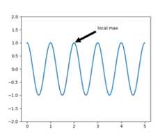
In this example, both thexy (arrow tip) andxytext locations(text location) are in data coordinates. There are a variety of othercoordinate systems one can choose – you can specify the coordinatesystem ofxy andxytext with one of the following strings forxycoords andtextcoords (default is ‘data’)
| argument | coordinate system |
|---|---|
| ‘figure points’ | points from the lower left corner of the figure |
| ‘figure pixels’ | pixels from the lower left corner of the figure |
| ‘figure fraction’ | 0,0 is lower left of figure and 1,1 is upper right |
| ‘axes points’ | points from lower left corner of axes |
| ‘axes pixels’ | pixels from lower left corner of axes |
| ‘axes fraction’ | 0,0 is lower left of axes and 1,1 is upper right |
| ‘data’ | use the axes data coordinate system |
For example to place the text coordinates in fractional axescoordinates, one could do:
ax.annotate('local max',xy=(3,1),xycoords='data',xytext=(0.8,0.95),textcoords='axes fraction',arrowprops=dict(facecolor='black',shrink=0.05),horizontalalignment='right',verticalalignment='top',)
For physical coordinate systems (points or pixels) the origin is thebottom-left of the figure or axes.
Optionally, you can enable drawing of an arrow from the text to the annotatedpoint by giving a dictionary of arrow properties in the optional keywordargumentarrowprops.
arrowprops key | description |
|---|---|
| width | the width of the arrow in points |
| frac | the fraction of the arrow length occupied by the head |
| headwidth | the width of the base of the arrow head in points |
| shrink | move the tip and base some percent away fromthe annotated point and text |
| **kwargs | any key formatplotlib.patches.Polygon,e.g.,facecolor |
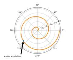
In the example below, thexy point is in native coordinates(xycoords defaults to ‘data’). For a polar axes, this is in(theta, radius) space. The text in this example is placed in thefractional figure coordinate system.matplotlib.text.Textkeyword args likehorizontalalignment,verticalalignment andfontsize are passed fromannotate to theText instance.
importnumpyasnpimportmatplotlib.pyplotaspltfig=plt.figure()ax=fig.add_subplot(111,polar=True)r=np.arange(0,1,0.001)theta=2*2*np.pi*rline,=ax.plot(theta,r,color='#ee8d18',lw=3)ind=800thisr,thistheta=r[ind],theta[ind]ax.plot([thistheta],[thisr],'o')ax.annotate('a polar annotation',xy=(thistheta,thisr),# theta, radiusxytext=(0.05,0.05),# fraction, fractiontextcoords='figure fraction',arrowprops=dict(facecolor='black',shrink=0.05),horizontalalignment='left',verticalalignment='bottom',)plt.show()
For more on all the wild and wonderful things you can do withannotations, including fancy arrows, seeAdvanced Annotationandpylab_examples example code: annotation_demo.py.
Do not proceed unless you have already readBasic annotation,text() andannotate()!
Let’s start with a simple example.
Thetext() function in the pyplot module (ortext method of the Axes class) takes bbox keyword argument, and whengiven, a box around the text is drawn.
bbox_props=dict(boxstyle="rarrow,pad=0.3",fc="cyan",ec="b",lw=2)t=ax.text(0,0,"Direction",ha="center",va="center",rotation=45,size=15,bbox=bbox_props)
The patch object associated with the text can be accessed by:
bb=t.get_bbox_patch()
The return value is an instance of FancyBboxPatch and the patchproperties like facecolor, edgewidth, etc. can be accessed andmodified as usual. To change the shape of the box, use theset_boxstylemethod.
bb.set_boxstyle("rarrow",pad=0.6)
The arguments are the name of the box style with its attributes askeyword arguments. Currently, following box styles are implemented.
Class Name Attrs Circle circlepad=0.3 DArrow darrowpad=0.3 LArrow larrowpad=0.3 RArrow rarrowpad=0.3 Round roundpad=0.3,rounding_size=None Round4 round4pad=0.3,rounding_size=None Roundtooth roundtoothpad=0.3,tooth_size=None Sawtooth sawtoothpad=0.3,tooth_size=None Square squarepad=0.3

Note that the attribute arguments can be specified within the stylename with separating comma (this form can be used as “boxstyle” valueof bbox argument when initializing the text instance)
bb.set_boxstyle("rarrow,pad=0.6")
Theannotate() function in the pyplot module(or annotate method of the Axes class) is used to draw an arrowconnecting two points on the plot.
ax.annotate("Annotation",xy=(x1,y1),xycoords='data',xytext=(x2,y2),textcoords='offset points',)
This annotates a point atxy in the given coordinate (xycoords)with the text atxytext given intextcoords. Often, theannotated point is specified in thedata coordinate and the annotatingtext inoffset points.Seeannotate() for available coordinate systems.
An arrow connecting two points (xy & xytext) can be optionally drawn byspecifying thearrowprops argument. To draw only an arrow, useempty string as the first argument.
ax.annotate("",xy=(0.2,0.2),xycoords='data',xytext=(0.8,0.8),textcoords='data',arrowprops=dict(arrowstyle="->",connectionstyle="arc3"),)

The arrow drawing takes a few steps.
connectionstyle key value.arrowstyle key value.
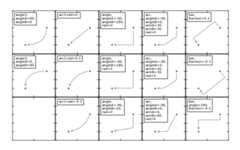
The creation of the connecting path between two points is controlled byconnectionstyle key and the following styles are available.
Name Attrs angleangleA=90,angleB=0,rad=0.0 angle3angleA=90,angleB=0 arcangleA=0,angleB=0,armA=None,armB=None,rad=0.0 arc3rad=0.0 bararmA=0.0,armB=0.0,fraction=0.3,angle=None
Note that “3” inangle3 andarc3 is meant to indicate that theresulting path is a quadratic spline segment (three controlpoints). As will be discussed below, some arrow style options can onlybe used when the connecting path is a quadratic spline.
The behavior of each connection style is (limitedly) demonstrated in theexample below. (Warning : The behavior of thebar style is currently notwell defined, it may be changed in the future).
The connecting path (after clipping and shrinking) is then mutated toan arrow patch, according to the givenarrowstyle.
Name Attrs -None ->head_length=0.4,head_width=0.2 -[widthB=1.0,lengthB=0.2,angleB=None |-|widthA=1.0,widthB=1.0 -|>head_length=0.4,head_width=0.2 <-head_length=0.4,head_width=0.2 <->head_length=0.4,head_width=0.2 <|-head_length=0.4,head_width=0.2 <|-|>head_length=0.4,head_width=0.2 fancyhead_length=0.4,head_width=0.4,tail_width=0.4 simplehead_length=0.5,head_width=0.5,tail_width=0.2 wedgetail_width=0.3,shrink_factor=0.5

Some arrowstyles only work with connection styles that generate aquadratic-spline segment. They arefancy,simple, andwedge.For these arrow styles, you must use the “angle3” or “arc3” connectionstyle.
If the annotation string is given, the patchA is set to the bbox patchof the text by default.

As in the text command, a box around the text can be drawn usingthebbox argument.

By default, the starting point is set to the center of the textextent. This can be adjusted withrelpos key value. The valuesare normalized to the extent of the text. For example, (0,0) meanslower-left corner and (1,1) means top-right.
There are classes of artists that can be placed at an anchored locationin the Axes. A common example is the legend. This type of artist canbe created by using the OffsetBox class. A few predefined classes areavailable inmpl_toolkits.axes_grid.anchored_artists.
frommpl_toolkits.axes_grid.anchored_artistsimportAnchoredTextat=AnchoredText("Figure 1a",prop=dict(size=8),frameon=True,loc=2,)at.patch.set_boxstyle("round,pad=0.,rounding_size=0.2")ax.add_artist(at)
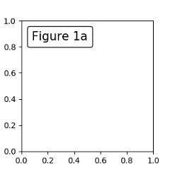
Theloc keyword has same meaning as in the legend command.
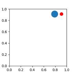
A simple application is when the size of the artist (or collection ofartists) is known in pixel size during the time of creation. Forexample, If you want to draw a circle with fixed size of 20 pixel x 20pixel (radius = 10 pixel), you can utilizeAnchoredDrawingArea. The instance is created with a size of thedrawing area (in pixels), and arbitrary artists can added to thedrawing area. Note that the extents of the artists that are added tothe drawing area are not related to the placement of the drawingarea itself. Only the initial size matters.
frommpl_toolkits.axes_grid.anchored_artistsimportAnchoredDrawingAreaada=AnchoredDrawingArea(20,20,0,0,loc=1,pad=0.,frameon=False)p1=Circle((10,10),10)ada.drawing_area.add_artist(p1)p2=Circle((30,10),5,fc="r")ada.drawing_area.add_artist(p2)
The artists that are added to the drawing area should not have atransform set (it will be overridden) and the dimensions of thoseartists are interpreted as a pixel coordinate, i.e., the radius of thecircles in above example are 10 pixels and 5 pixels, respectively.
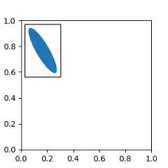
Sometimes, you want your artists to scale with the data coordinate (orcoordinates other than canvas pixels). You can useAnchoredAuxTransformBox class. This is similar toAnchoredDrawingArea except that the extent of the artist isdetermined during the drawing time respecting the specified transform.
frommpl_toolkits.axes_grid.anchored_artistsimportAnchoredAuxTransformBoxbox=AnchoredAuxTransformBox(ax.transData,loc=2)el=Ellipse((0,0),width=0.1,height=0.4,angle=30)# in data coordinates!box.drawing_area.add_artist(el)
The ellipse in the above example will have width and heightcorresponding to 0.1 and 0.4 in data coordinateing and will beautomatically scaled when the view limits of the axes change.
As in the legend, the bbox_to_anchor argument can be set. Using theHPacker and VPacker, you can have an arrangement(?) of artist as in thelegend (as a matter of fact, this is how the legend is created).

Note that unlike the legend, thebbox_transform is setto IdentityTransform by default.
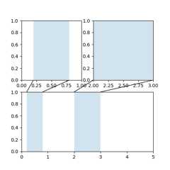
The Annotation in matplotlib supports several types of coordinates asdescribed inBasic annotation. For an advanced user who wantsmore control, it supports a few other options.
Transforminstance. For example,ax.annotate("Test",xy=(0.5,0.5),xycoords=ax.transAxes)is identical to
ax.annotate("Test",xy=(0.5,0.5),xycoords="axes fraction")With this, you can annotate a point in other axes.
ax1,ax2=subplot(121),subplot(122)ax2.annotate("Test",xy=(0.5,0.5),xycoords=ax1.transData,xytext=(0.5,0.5),textcoords=ax2.transData,arrowprops=dict(arrowstyle="->"))
Artistinstance. The xy value (orxytext) is interpreted as a fractional coordinate of the bbox(return value ofget_window_extent) of the artist.an1=ax.annotate("Test 1",xy=(0.5,0.5),xycoords="data",va="center",ha="center",bbox=dict(boxstyle="round",fc="w"))an2=ax.annotate("Test 2",xy=(1,0.5),xycoords=an1,# (1,0.5) of the an1's bboxxytext=(30,0),textcoords="offset points",va="center",ha="left",bbox=dict(boxstyle="round",fc="w"),arrowprops=dict(arrowstyle="->"))Note that it is your responsibility that the extent of thecoordinate artist (an1 in above example) is determined beforean2gets drawn. In most cases, it means thatan2 needs to be drawnlater thanan1.
A callable object that returns an instance of either
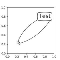
BboxBaseorTransform. If a transform isreturned, it is the same as 1 and if a bbox is returned, it is the sameas 2. The callable object should take a single argument of therenderer instance. For example, the following two commands giveidentical resultsan2=ax.annotate("Test 2",xy=(1,0.5),xycoords=an1,xytext=(30,0),textcoords="offset points")an2=ax.annotate("Test 2",xy=(1,0.5),xycoords=an1.get_window_extent,xytext=(30,0),textcoords="offset points")A tuple of two coordinate specifications. The first item is for thex-coordinate and the second is for the y-coordinate. For example,
annotate("Test",xy=(0.5,1),xycoords=("data","axes fraction"))0.5 is in data coordinates, and 1 is in normalized axes coordinates.You may use an artist or transform as with a tuple. For example,
importmatplotlib.pyplotaspltplt.figure(figsize=(3,2))ax=plt.axes([0.1,0.1,0.8,0.7])an1=ax.annotate("Test 1",xy=(0.5,0.5),xycoords="data",va="center",ha="center",bbox=dict(boxstyle="round",fc="w"))an2=ax.annotate("Test 2",xy=(0.5,1.),xycoords=an1,xytext=(0.5,1.1),textcoords=(an1,"axes fraction"),va="bottom",ha="center",bbox=dict(boxstyle="round",fc="w"),arrowprops=dict(arrowstyle="->"))plt.show()Sometimes, you want your annotation with some “offset points”, not from theannotated point but from some other point.
OffsetFromis a helper class for such cases.importmatplotlib.pyplotaspltplt.figure(figsize=(3,2))ax=plt.axes([0.1,0.1,0.8,0.7])an1=ax.annotate("Test 1",xy=(0.5,0.5),xycoords="data",va="center",ha="center",bbox=dict(boxstyle="round",fc="w"))frommatplotlib.textimportOffsetFromoffset_from=OffsetFrom(an1,(0.5,0))an2=ax.annotate("Test 2",xy=(0.1,0.1),xycoords="data",xytext=(0,-10),textcoords=offset_from,# xytext is offset points from "xy=(0.5, 0), xycoords=an1"va="top",ha="center",bbox=dict(boxstyle="round",fc="w"),arrowprops=dict(arrowstyle="->"))plt.show()You may take a look at this examplepylab_examples example code: annotation_demo3.py.
The ConnectorPatch is like an annotation without text. While the annotatefunction is recommended in most situations, the ConnectorPatch is useful whenyou want to connect points in different axes.
frommatplotlib.patchesimportConnectionPatchxy=(0.2,0.2)con=ConnectionPatch(xyA=xy,xyB=xy,coordsA="data",coordsB="data",axesA=ax1,axesB=ax2)ax2.add_artist(con)
The above code connects point xy in the data coordinates ofax1 topoint xy in the data coordinates ofax2. Here is a simple example.

While the ConnectorPatch instance can be added to any axes, you may want to addit to the axes that is latest in drawing order to prevent overlap by otheraxes.
mpl_toolkits.axes_grid.inset_locator defines some patch classes usefulfor interconnecting two axes. Understanding the code requires someknowledge of how mpl’s transform works. But, utilizing it will bestraight forward.
You can use a custom box style. The value for theboxstyle can be acallable object in the following forms.:
def__call__(self,x0,y0,width,height,mutation_size,aspect_ratio=1.):""" Given the location and size of the box, return the path of the box around it. - *x0*, *y0*, *width*, *height* : location and size of the box - *mutation_size* : a reference scale for the mutation. - *aspect_ratio* : aspect-ratio for the mutation. """path=...returnpath
Here is a complete example.

However, it is recommended that you derive from thematplotlib.patches.BoxStyle._Base as demonstrated below.
frommatplotlib.pathimportPathfrommatplotlib.patchesimportBoxStyleimportmatplotlib.pyplotasplt# we may derive from matplotlib.patches.BoxStyle._Base class.# You need to override transmute method in this case.classMyStyle(BoxStyle._Base):""" A simple box. """def__init__(self,pad=0.3):""" The arguments need to be floating numbers and need to have default values. *pad* amount of padding """self.pad=padsuper(MyStyle,self).__init__()deftransmute(self,x0,y0,width,height,mutation_size):""" Given the location and size of the box, return the path of the box around it. - *x0*, *y0*, *width*, *height* : location and size of the box - *mutation_size* : a reference scale for the mutation. Often, the *mutation_size* is the font size of the text. You don't need to worry about the rotation as it is automatically taken care of. """# paddingpad=mutation_size*self.pad# width and height with padding added.width,height=width+2.*pad, \height+2.*pad,# boundary of the padded boxx0,y0=x0-pad,y0-pad,x1,y1=x0+width,y0+heightcp=[(x0,y0),(x1,y0),(x1,y1),(x0,y1),(x0-pad,(y0+y1)/2.),(x0,y0),(x0,y0)]com=[Path.MOVETO,Path.LINETO,Path.LINETO,Path.LINETO,Path.LINETO,Path.LINETO,Path.CLOSEPOLY]path=Path(cp,com)returnpath# register the custom styleBoxStyle._style_list["angled"]=MyStyleplt.figure(1,figsize=(3,3))ax=plt.subplot(111)ax.text(0.5,0.5,"Test",size=30,va="center",ha="center",rotation=30,bbox=dict(boxstyle="angled,pad=0.5",alpha=0.2))delBoxStyle._style_list["angled"]plt.show()

Similarly, you can define a custom ConnectionStyle and a custom ArrowStyle.See the source code oflib/matplotlib/patches.py and checkhow each style class is defined.


